2 Ordinary Differential Equations
Papula (2015) gives an introduction to the topic in Part IV, Chapter 1, “Gewöhnliche Differentialgleichungen” (ordinary differential equations).
Definition 2.1 (Ordinary Differential Equation) A differential equation is a relation between an unknown function \(y(x)\), its independent variable \(x\), and an arbitrary number of its derivatives. An ordinary differential equation (ODE) is a differential equation in which the independent variable, and hence the derivatives, are one-dimensional. We assume that an ODE can be written in the explicit form \[ \frac{\mathrm{d}^{n}y}{\mathrm{d}x^{n}} = f\left(x, y, \frac{\mathrm{d}y}{\mathrm{d}x}, \frac{\mathrm{d}^2y}{\mathrm{d}x^2}, \dots, \frac{\mathrm{d}^{n-1}y}{\mathrm{d}x^{n-1}}\right), \quad \text{for short} \quad y^{(n)} = f\left(x, y, y', \dots, y^{(n-1)}\right), \] where \(f\) is an arbitrary function of some or all of its arguments. The highest order of derivative \(n\) that occurs is called the order of the ODE.
Remark 2.1 (Memory Aid for Integration by Parts). Not entirely correct mathematically, but easy to remember: \[ \int u' v = uv - \int u v' \]
Table 2.1 summarizes the symbols of this chapter. Up to Section 2.7, \(x\) denotes the independent variable and \(a, b\) denote the coefficients of a general linear ODE. From Section 2.7 onward, \(t\) is the independent variable, \(x(t)\) the displacement, and \(b\) the damper constant. Likewise, \(A\) first stands for a scalar amplitude and only in Section 2.9 for a matrix.
| Symbol | Meaning | Type | Defined in |
|---|---|---|---|
| General Theory | |||
| \(a\) | Constant coefficient of a linear ODE (\(y' + ay = g(x)\); growth rate in \(y' = ay\)) | Constant | Equation 2.3 |
| \(a, b\) | Constant coefficients of the general linear second-order ODE \(y'' + ay' + by = g(x)\) | Constant | Definition 2.7 |
| \(\mathrm{d}\) | Differential (\(\mathrm{d}x\), \(\frac{\mathrm{d}y}{\mathrm{d}x}\)) | Operator | Definition 2.1 |
| \(\mathrm{e}\) | Euler’s number | Constant | Example 2.1 |
| \(f\) | Function; right-hand side of the ODE \(y' = f(x,y)\) or \(y^{(n)} = f(x, y, \dots, y^{(n-1)})\) | Function | Definition 2.1 |
| \(f(x)\) | Coefficient function of the linear ODE \(y' + f(x)y = g(x)\) | Function | Definition 2.6 |
| \(g(x)\) | Forcing function of a linear ODE; as a vector \(g(x)\) or \(g(t)\) for systems | Function | Definition 2.6 |
| \(\mathrm{j}\) | Imaginary unit, \(\mathrm{j}^2 = -1\) | Constant | Proposition 2.2 |
| \(n\) | Order of an ODE; dimension of a matrix or system | Index | Definition 2.1 |
| \(x\) | Independent variable | Scalar | Definition 2.1 |
| \(x_0\), \(y_0\) | Initial point; initial value \(y(x_0)\) | Scalar | Definition 2.3 |
| \(y\) | Unknown function \(y(x)\) or vector of unknown functions | Function | Definition 2.1 |
| \(y_{\mathrm{h}}, y_{\mathrm{p}}\) | General solution of the homogeneous ODE and particular solution, respectively | Function | Theorem 2.2 |
| \(y_1, y_2\) | Basis solutions of a homogeneous linear second-order ODE | Function | Definition 2.8 |
| \(C\); \(C_1, C_2\) | Constant of integration; \(C_1, \dots, C_n\) constants of integration or coefficients of the general solution | Constant | Example 2.1 |
| \(C_0\) | Combined constant of integration of the general solution | Constant | Example 2.2 |
| \(K(x)\) | Factor function that replaces \(C\) in the variation of constants | Function | Section 2.2.1 |
| \(W\) | Wronskian \(W(y_1; y_2)\) | Function | Definition 2.8 |
| \(\mathbb{R}\), \(\mathbb{C}\) | Set of real and of complex numbers, respectively | Set | Example 2.2 |
| \(\alpha\) | Real part of a complex eigenvalue, \(\lambda_{1,2} = \alpha \pm \mathrm{j}\omega\) | Scalar | Proposition 2.2 |
| \(\beta\) | Angular frequency of the forcing function \(g(x) = \sin(\beta x)\) | Constant | Equation 2.6 |
| \(\lambda\); \(\lambda_{1,2}\) | Eigenvalue or root of the characteristic equation (exponent in the ansatz \(\mathrm{e}^{\lambda t}\)); \(\lambda_{1,2}\) the two roots | Scalar | Section 2.3 |
| \(\varphi\) | Phase angle (initial phase angle) of an oscillation; \(\varphi_{\mathrm{d}}\) of the damped oscillation; \(\varphi(\omega)\) phase response | Scalar | Equation 2.6 |
| \(\omega\) | Angular frequency (excitation angular frequency; imaginary part of an eigenvalue) | Scalar | Proposition 2.2 |
| \(y', y'', y^{(n)}\) | First, second, \(n\)-th derivative with respect to the independent variable | Operator | Definition 2.1 |
| \(\frac{\partial}{\partial x}\) | Partial derivative | Operator | Definition 2.5 |
| \(\int \dots \mathrm{d}x\) | Integral | Operator | Example 2.2 |
| \(\lvert z \rvert\) | Absolute value | Operator | Example 2.2 |
| local | \(g(y)\) in Definition 2.4; \(a, b, c\) and \(u\) in Theorem 2.1; \(u\) in Proposition 2.1; \(g(x;y)\), \(h(x;y)\), \(u(x;y)\) in Definition 2.5; \(K(y)\) in Example 2.7; ansatz coefficients \(a_0, a_1, a_2\), \(A\), \(B\); boundary points \(x_1, \dots, x_n\) in Definition 2.3 | local | where used |
| Oscillations, Pendulums, Reduction of Order | |||
| \(b\) | Damper constant of the mass-spring oscillator | Constant | Definition 2.9 |
| \(c\) | Spring constant | Constant | Theorem 2.7 |
| \(g\) | Gravitational acceleration | Constant | Section 2.8 |
| \(i\) | Running index (component) | Index | Section 2.9 |
| \(l\) | Length of the simple pendulum | Constant | Definition 2.13 |
| \(m\) | Mass | Constant | Theorem 2.6 |
| \(r(t), w(t)\) | Population of rabbits and of wolves, respectively | Function | Example 2.47 |
| \(s(t)\) | Arc length of the simple pendulum | Function | Section 2.8 |
| \(t\) | Time | Scalar | Theorem 2.6 |
| \(t_1, t_2\) | Time of the turning point in the overdamped case and in the aperiodic limiting case, respectively | Scalar | Figure 2.10, Figure 2.13 |
| \(v\), \(v_0\) | Velocity, \(v = \dot{x}\); \(v_0\) initial velocity | Scalar | Definition 2.9 |
| \(x(t)\), \(x_0\) | Displacement from the rest position; \(x_0\) initial displacement | Function | Theorem 2.7 |
| \(x_{\mathrm{h}}, x_{\mathrm{p}}\) | Homogeneous and particular component of the oscillation solution, respectively | Function | Equation 2.24 |
| \(x_{\mathrm{st}}\) | Static displacement, \(x_{\mathrm{st}} = F_0/c\) | Scalar | Definition 2.12 |
| \(\underline{x}_{\mathrm{p}}\) | Complex particular solution (underline = complex quantity) | Function | Equation 2.18 |
| \(y_1, \dots, y_n\) | Components of the state vector \(S\) in the reduction of order (\(y_1 = y\), \(y_2 = y'\), …) | Function | Theorem 2.14 |
| \(z\) | Complex number | Scalar | Figure 2.14 |
| \(A\), \(A(\omega)\) | Amplitude of an oscillation; \(A(\omega)\) amplitude frequency response, \(A_{\mathrm{r}} = A_{\max}\) resonance amplitude | Scalar | Section 2.7.2 |
| \(A\) | Matrix (coefficient or system matrix); \(a_1, \dots, a_n\) entries of its last row | Matrix | Section 2.9 |
| \(A_{\mathrm{d}}\) | Amplitude of the damped oscillation \(x(t) = A_{\mathrm{d}}\,\mathrm{e}^{-\delta t}\sin(\omega_{\mathrm{d}} t + \varphi_{\mathrm{d}})\) | Scalar | Theorem 2.10 |
| \(F\) | Force; \(F(t)\) external force, \(F_0\) its amplitude, \(F_1, F_2, F_3\) component forces, \(F_{\mathrm{R}}\) restoring force, \(F_{\mathrm{G}}\) weight | Scalar | Theorem 2.6 |
| \(\underline{F}(t)\) | Complex excitation force | Function | Equation 2.19 |
| \(K_0\) | Excitation amplitude per unit mass, \(K_0 = F_0/m\) | Constant | Equation 2.17 |
| \(S\) | State vector \(S(t)\); \(S_i\) its \(i\)-th component | Vector | Section 2.9 |
| \(T\) | Period of oscillation; \(T_0\) of the simple pendulum, \(T_{\mathrm{d}}\) of the damped oscillation | Scalar | Section 2.7.2 |
| \(\delta\) | Damping factor or decay constant, \(\delta = b/(2m)\); \(\delta_1, \delta_2, \delta_3\) sample values | Constant | Equation 2.10 |
| \(\Delta\) | Discriminant of the characteristic equation, \(\Delta = \delta^2 - \omega_0^2\) | Scalar | Equation 2.11 |
| \(\nu_0\) | Frequency of the simple pendulum, \(\nu_0 = \omega_0/(2\pi)\) | Scalar | Section 2.8 |
| \(\pi\) | The number pi (italic, KaTeX exception) | Constant | Section 2.7.2 |
| \(\varphi(t)\), \(\varphi_0\) | Angle of deflection of the simple pendulum; \(\varphi_0\) initial deflection | Function | Definition 2.13 |
| \(\Psi(\omega)\) | Radicand of the resonance curve, \(\Psi(\omega) = (\omega_0^2 - \omega^2)^2 + (2\delta\omega)^2\) | Function | Section 2.7.7.1 |
| \(\omega_0\) | Natural angular frequency of the undamped single-mass oscillator, \(\omega_0 = \sqrt{c/m}\) (simple pendulum: \(\sqrt{g/l}\)) | Constant | Equation 2.8 |
| \(\omega_{\mathrm{d}}\) | Natural angular frequency of the damped oscillation, \(\omega_{\mathrm{d}} = \sqrt{\omega_0^2 - \delta^2}\) | Constant | Theorem 2.10 |
| \(\omega_{\mathrm{r}}\) | Resonance angular frequency, \(\omega_{\mathrm{r}} = \sqrt{\omega_0^2 - 2\delta^2}\) | Constant | Theorem 2.13 |
| \(\dot{x}, \ddot{x}\) | First and second derivative with respect to time \(t\) | Operator | Theorem 2.6 |
| \(\operatorname{Im}\) | Imaginary part | Operator | Section 2.7.6 |
| \(^T\) | Transpose | Operator | Example 2.49 |
| local | Bodies 1, 2 in Theorem 2.6; turning points \(A, B\) in Figure 2.22 | local | where used |
The solutions of an ODE form a family from which additional conditions select a single solution.
Definition 2.2 (General and Particular Solution) The general solution of an ODE of order \(n\) comprises all solutions of the equation. In general, it contains \(n\) undetermined constants of integration and describes a family of functions. A particular solution is a member of this family in which the constants have fixed values.
The constants cannot be determined from the ODE itself, but only from additional conditions such as initial or boundary conditions. A particular solution then satisfies both the ODE and these requirements.
Example 2.1 (General and Particular Solution) The first-order ODE \[ \frac{\mathrm{d}y}{\mathrm{d}x} = 3y \] has the general solution \(y = C\mathrm{e}^{3x}\) with an arbitrary constant \(C\). It describes a family of exponential functions whose curves depend on the value of \(C\). If \(y(0) = 4\) is additionally required, substituting into the general solution yields \(4 = C\mathrm{e}^{0} = C\). The particular solution is therefore \(y = 4\mathrm{e}^{3x}\).
Definition 2.3 (Initial Value Problem and Boundary Value Problem) In an initial value problem, the function value and the values of the first \(n-1\) derivatives of the solution \(y = y(x)\) of an ODE of order \(n\) are prescribed at a point \(x_0\): \[ y(x_0) = y_0, \quad y'(x_0) = y_0', \quad y''(x_0) = y_0'', \quad \dots, \quad y^{(n-1)}(x_0) = y_0^{(n-1)}. \] In a boundary value problem, the function values \(y(x_1), y(x_2), \dots, y(x_n)\) of the solution are prescribed at \(n\) different points \(x_1, x_2, \dots, x_n\).
2.1 First-Order Differential Equations
2.1.1 Separation of Variables
Definition 2.4 (Separable ODE) A first-order ODE of the form \[ y' = \frac{\mathrm{d}y}{\mathrm{d}x} = f(x)\,g(y) \] is called separable (ODE with separable variables).
It is solved by separating the variables \(x\) and \(y\) onto the two sides of the equation, integrating both sides, and solving the result for \(y\). The antiderivatives required for this are collected in Table A.1.
Example 2.2 (Separation of Variables) The ODE \(y' = y\) can be solved for \(y \neq 0\) by separation of variables: \[ \frac{\mathrm{d}y}{\mathrm{d}x} = y \Rightarrow \frac{\mathrm{d}y}{y} = \mathrm{d}x \Rightarrow \int \frac{\mathrm{d}y}{y} = \int \mathrm{d}x \Rightarrow \ln\lvert y\rvert = x + C. \] The constants of integration arising on both sides have been combined into a single constant. The solution is now in implicit form. Solving for \(y\) yields \[ \lvert y\rvert = \mathrm{e}^{x+C} = \mathrm{e}^C \mathrm{e}^x \Rightarrow y = \pm \mathrm{e}^C \mathrm{e}^x. \] When \(C\) runs through all real numbers, \(\mathrm{e}^C\) runs through all positive and \(\pm\mathrm{e}^C\) through all nonzero real numbers. We set \[ y = \pm \mathrm{e}^C \mathrm{e}^x = C_0 \mathrm{e}^x, \quad C_0 = \pm \mathrm{e}^C \neq 0. \] Since \(y = 0\) also solves the ODE \(y' = y\), the general solution is \[ y = C_0 \mathrm{e}^x, \quad C_0 \in \mathbb{R}. \]
Remark 2.2 (Logarithmic Terms). If logarithmic terms such as \(\ln\lvert y\rvert\) in the example above arise when integrating an ODE, it is convenient to write the constant of integration \(C\) in the form \(\ln\lvert C\rvert\). This is possible because, as \(C\) runs through all real numbers, so does \(\ln\lvert C\rvert\), see Figure 2.1.
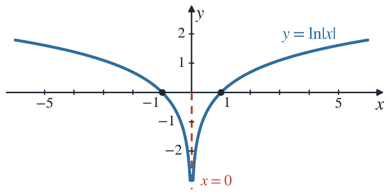
With this note, we solve the ODE \(y' = y\) once more. After separating the variables and integrating, we write the constant of integration as \(\ln\lvert C\rvert\) with \(C \neq 0\): \[ \frac{\mathrm{d}y}{\mathrm{d}x} = y \Rightarrow \frac{\mathrm{d}y}{y} = \mathrm{d}x \Rightarrow \int \frac{\mathrm{d}y}{y} = \int \mathrm{d}x \Rightarrow \ln\lvert y\rvert = x + \ln\lvert C\rvert. \] The logarithmic terms are combined, \[ \ln\lvert y\rvert - \ln\lvert C\rvert = \ln \left\lvert\frac{y}{C}\right\rvert = x, \] and taking the exponential yields \[ \left\lvert \frac{y}{C} \right\rvert = \mathrm{e}^x \Rightarrow \frac{y}{C} = \pm \mathrm{e}^x \Rightarrow y = \pm C \mathrm{e}^x. \] With \(C_0 = \pm C\) and including the solution \(y = 0\), the general solution of the ODE \(y' = y\) is therefore again \[ y = C_0 \mathrm{e}^x, \quad C_0 \in \mathbb{R}. \]
Example 2.3 (Separation of Variables with an Initial Value) We solve the initial value problem \[ x + xy' = 0, \qquad y(0) = 2. \] For \(x \neq 0\), we divide by \(x\) and obtain \(1 + y' = 0\), that is, \[ \frac{\mathrm{d}y}{\mathrm{d}x} = -1. \] The right-hand side depends neither on \(x\) nor on \(y\), so the variables are already separated. Integrating both sides of \(\mathrm{d}y = -\mathrm{d}x\) yields \[ \int \mathrm{d}y = -\int \mathrm{d}x \Rightarrow y = -x + C, \quad C \in \mathbb{R}. \] The initial condition \(y(0) = C = 2\) gives the solution of the initial value problem \[ y = 2 - x. \] Check: with \(y' = -1\), we have \(x + x \cdot (-1) = 0\) for all \(x\), hence also at \(x = 0\), where we were not allowed to divide by \(x\).
Example 2.4 (Separation of Variables with a Singular Solution) We determine the general solution of the ODE \[ y' + y^2 = 0. \] For \(y \neq 0\), we separate the variables and integrate: \[ \frac{\mathrm{d}y}{\mathrm{d}x} = -y^2 \Rightarrow -\frac{\mathrm{d}y}{y^2} = \mathrm{d}x \Rightarrow -\int \frac{\mathrm{d}y}{y^2} = \int \mathrm{d}x \Rightarrow \frac{1}{y} = x + C. \] Solving for \(y\) yields the general solution \[ y = \frac{1}{x + C}, \quad C \in \mathbb{R}. \] Check: \(y' = -\frac{1}{(x+C)^2} = -y^2\). Each of these solutions is defined only on an interval that does not contain the pole \(x = -C\).
In separating the variables, we divided by \(y^2\) and thereby excluded the case \(y = 0\). The zero function \(y = 0\) also solves the ODE, but it is not contained in the family of solutions for any value of \(C\). Such a solution is called singular. It must be stated separately.
2.1.2 Integration of a Differential Equation by Substitution
Theorem 2.1 (Integration of an ODE by Substitution) A first-order ODE of the type \[ y' = f(ax+by+c) \] is transformed by the substitution \[ u = ax+by+c \tag{2.1}\] into the separable ODE \[ u' = a + b f(u) \] for the auxiliary function \(u = u(x)\).
Proof. Differentiating Equation 2.1 with respect to \(x\) yields \(u' = a + by'\). With \(y' = f(ax+by+c) = f(u)\) it follows that \[ u' = \frac{\mathrm{d}u}{\mathrm{d}x} = a + b f(u). \] The right-hand side depends only on \(u\), so this ODE can be solved by separation of the variables \(x\) and \(u\).
The solution \(u = u(x)\) is then substituted into Equation 2.1, and the equation is solved for \(y\).
Proposition 2.1 (Substitution \(u = y/x\)) A first-order ODE of the type \[ y' = f\left(\frac{y}{x}\right) \] is transformed by the substitution \(u = y/x\), i.e., \(y = xu\), into the separable ODE \[ u + xu' = f(u) \] for the auxiliary function \(u = u(x)\).
Proof. Differentiating \(y = xu\) with respect to \(x\) yields \(y' = u'x + u\). Since \(y' = f(y/x) = f(u)\), the claim follows.
Both substitutions follow the same procedure: carry out the substitution, integrate the ODE for the auxiliary function \(u = u(x)\) by separation of variables, undo the substitution, and solve the equation for \(y\).
Example 2.5 (Substitution \(u = ax + by + c\)) We solve the ODE \[ y' = 2x - y. \] The right-hand side has the form \(f(ax+by+c)\) with \(a = 2\), \(b = -1\), \(c = 0\), and \(f(u) = u\). By Theorem 2.1, the substitution \[ u = 2x - y, \qquad u' = 2 - y', \] leads to the separable ODE \[ u' = 2 - u. \] For \(u \neq 2\), we separate the variables and write the constant of integration as \(-\ln\lvert C\rvert\): \[ \frac{\mathrm{d}u}{2 - u} = \mathrm{d}x \Rightarrow -\ln\lvert 2 - u\rvert = x - \ln\lvert C\rvert \Rightarrow \ln\left\lvert \frac{2 - u}{C} \right\rvert = -x. \] Taking exponentials yields \(2 - u = C\mathrm{e}^{-x}\), where the sign is absorbed into the constant \(C\). The value \(C = 0\) gives the initially excluded solution \(u = 2\). Hence \[ u = 2 - C\mathrm{e}^{-x}, \quad C \in \mathbb{R}. \] The back-substitution \(y = 2x - u\) yields the general solution \[ y = 2x - 2 + C\mathrm{e}^{-x}, \quad C \in \mathbb{R}. \] Check: \(y' = 2 - C\mathrm{e}^{-x}\) and \(2x - y = 2x - (2x - 2 + C\mathrm{e}^{-x}) = 2 - C\mathrm{e}^{-x}\).
Example 2.6 (Substitution \(u = y/x\)) We solve the ODE \[ y' = \frac{x+2y}{x} \qquad (x \neq 0). \] Splitting the right-hand side yields \[ y' = 1 + 2\,\frac{y}{x}, \] that is, the type \(y' = f(y/x)\) with \(f(u) = 1 + 2u\). By Proposition 2.1, the substitution \(u = y/x\), i.e., \(y = xu\), leads to \[ u + xu' = 1 + 2u \Rightarrow xu' = 1 + u. \] For \(u \neq -1\), we separate the variables and write the constant of integration as \(\ln\lvert C\rvert\): \[ \frac{\mathrm{d}u}{1 + u} = \frac{\mathrm{d}x}{x} \Rightarrow \ln\lvert 1 + u\rvert = \ln\lvert x\rvert + \ln\lvert C\rvert = \ln\lvert Cx\rvert. \] Taking exponentials yields \(1 + u = Cx\), where the sign is again absorbed into \(C\). The value \(C = 0\) gives the initially excluded solution \(u = -1\). Hence \(u = Cx - 1\), and the back-substitution \(y = xu\) yields the general solution \[ y = Cx^2 - x, \quad C \in \mathbb{R}. \] Check: \(y' = 2Cx - 1\) and \[ \frac{x + 2(Cx^2 - x)}{x} = \frac{2Cx^2 - x}{x} = 2Cx - 1. \]
2.1.3 Exact Differential Equations
Definition 2.5 (Exact ODE) A first-order ODE of the form \[ g(x;y)\, \mathrm{d}x + h(x;y)\, \mathrm{d}y = 0, \tag{2.2}\] in another notation \[ y' = -\frac{g(x;y)}{h(x;y)}, \] is called exact if the integrability condition \[ \frac{\partial g}{\partial y} = \frac{\partial h}{\partial x} \] is satisfied.
The continuous factor functions \(g(x;y)\) and \(h(x;y)\) of an exact ODE Equation 2.2 are the partial derivatives of an unknown function \(u(x;y)\): \[ \frac{\partial u}{\partial x} = g(x;y) \quad \text{and} \quad \frac{\partial u}{\partial y} = h(x;y). \] From these relations, \(u(x;y)\) is determined by indefinite integration. The general solution of the exact ODE Equation 2.2 is then given in the implicit form \[ u(x;y) = C \] where \(C\) is a constant of integration.
Example 2.7 (Exact Differential Equation) We solve the ODE \[ y' = \frac{\mathrm{d}y}{\mathrm{d}x} = \frac{2x+y}{y-x}. \] Multiplying by \((y - x)\,\mathrm{d}x\) yields \((y - x)\,\mathrm{d}y = (2x + y)\,\mathrm{d}x\). Bringing all terms to one side, we obtain the form Equation 2.2, \[ (2x + y)\,\mathrm{d}x + (x - y)\,\mathrm{d}y = 0, \] with the factor functions \[ g(x;y) = 2x + y \quad \text{and} \quad h(x;y) = x - y. \] The integrability condition is satisfied, \[ \frac{\partial g}{\partial y} = 1 = \frac{\partial h}{\partial x}, \] so the ODE is exact. We determine \(u(x;y)\) in two steps. Integrating \(\partial u/\partial x = g(x;y)\) with respect to \(x\) yields \[ u(x;y) = \int (2x + y)\,\mathrm{d}x = x^2 + xy + K(y), \] where the constant of integration \(K(y)\) may still depend on \(y\). Differentiating with respect to \(y\) and comparing with \(h(x;y)\) gives \[ \frac{\partial u}{\partial y} = x + K'(y) = x - y \Rightarrow K'(y) = -y \Rightarrow K(y) = -\frac{y^2}{2}. \] We may omit an additive constant in \(K(y)\) because it is absorbed into the constant \(C\) of the solution. Thus \[ u(x;y) = x^2 + xy - \frac{y^2}{2}, \] and the general solution in implicit form reads \[ x^2 + xy - \frac{y^2}{2} = C, \quad C \in \mathbb{R}. \] Solving this quadratic equation for \(y\) yields the explicit form \[ y = x \pm \sqrt{3x^2 - 2C}. \] Check: implicit differentiation of \(u(x;y) = C\) with respect to \(x\) yields \(2x + y + xy' - yy' = 0\), hence \(y'(y - x) = 2x + y\), which is the given ODE.
2.2 Linear First-Order Differential Equations
Definition 2.6 (Linear First-Order ODE) A first-order ODE is called linear if it can be written in the form \[ y' + f(x)\, y = g(x) \] The function \(f(x)\) is called the coefficient function, the function \(g(x)\) the forcing function. If the forcing function is absent, the ODE is called homogeneous, otherwise inhomogeneous.
The homogeneous linear first-order ODE \[ y' + f(x)\, y = 0 \] is separable. Separation of variables yields the general solution \[ y = C \mathrm{e}^{-\int f(x)\, \mathrm{d}x}, \quad C \in \mathbb{R}. \]
The following two examples follow Papula (2015, sec. IV.2.5.2).
Example 2.8 (Homogeneous Linear First-Order ODE) We seek the general solution of \[ x^2 y' + y = 0 \quad \text{or} \quad y' + \frac{1}{x^2}\, y = 0, \qquad x \neq 0. \] For \(y \neq 0\), separation of variables yields \[ \frac{\mathrm{d}y}{\mathrm{d}x} = -\frac{y}{x^2} \Rightarrow \frac{\mathrm{d}y}{y} = -\frac{\mathrm{d}x}{x^2}. \] Integrating both sides gives \[ \int \frac{\mathrm{d}y}{y} = -\int x^{-2}\, \mathrm{d}x \Rightarrow \ln\lvert y\rvert = \frac{1}{x} + \ln\lvert K\rvert, \quad K \neq 0, \] i.e., \(\ln\lvert y/K\rvert = 1/x\) and hence \(y/K = \pm\mathrm{e}^{1/x}\). With \(C = \pm K\), the general solution is \[ y = C \mathrm{e}^{1/x}, \quad C \in \mathbb{R}. \] The trivial solution \(y = 0\) is included as the special case \(C = 0\).
Example 2.9 (Homogeneous Linear First-Order ODE with an Initial Value) We seek the solution of the initial value problem \[ y' - 2xy = 0, \qquad y(0) = 5. \] Separation of variables yields \[ \frac{\mathrm{d}y}{\mathrm{d}x} = 2xy \Rightarrow \frac{\mathrm{d}y}{y} = 2x\, \mathrm{d}x \Rightarrow \int \frac{\mathrm{d}y}{y} = \int 2x\, \mathrm{d}x \Rightarrow \ln\lvert y\rvert = x^2 + \ln\lvert C\rvert, \] i.e., \(\ln\lvert y/C\rvert = x^2\) and hence the general solution \[ y = C \mathrm{e}^{x^2}, \quad C \in \mathbb{R}. \] The initial value gives \(y(0) = C \mathrm{e}^{0} = C = 5\). The initial value problem therefore has the solution \[ y = 5 \mathrm{e}^{x^2}. \]
2.2.1 Variation of Constants
An inhomogeneous linear first-order ODE \[ y' + f(x)\, y = g(x) \] is solved by variation of constants in two steps. First, the associated homogeneous ODE \(y' + f(x)\,y = 0\) is integrated by separation of variables: \[ y_{\mathrm{h}} = C \mathrm{e}^{-\int f(x)\, \mathrm{d}x}, \quad C \in \mathbb{R}. \] Then the constant of integration \(C\) is replaced by a still unknown function \(K(x)\). Substituting the ansatz \[ y = K(x)\, \mathrm{e}^{-\int f(x)\, \mathrm{d}x} \] into the inhomogeneous ODE yields a simple first-order ODE for the factor function \(K(x)\), which is solved by indefinite integration (antiderivatives in Table A.1).
The following two examples follow Papula (2015, sec. IV.2.5.3.1).
Example 2.10 (Variation of Constants) We seek the general solution of \[ y' + \frac{y}{x} = \cos(x), \qquad x \neq 0. \] Separation of variables yields the general solution of the homogeneous ODE, \[ y_{\mathrm{h}} = \frac{C}{x}, \quad C \in \mathbb{R}. \] Variation of constants leads to the ansatz \[ y = K(x)\, \frac{1}{x} \] with the derivative \[ y' = K'(x)\, \frac{1}{x} - K(x)\, \frac{1}{x^2} = \frac{K'(x)}{x} - \frac{K(x)}{x^2}. \] Substituting into the inhomogeneous ODE yields \[ K'(x) = x \cos(x) \Rightarrow K(x) = \int x \cos(x)\, \mathrm{d}x. \] Integration by parts yields \[ K(x) = \cos(x) + x \sin(x) + C_0, \quad C_0 \in \mathbb{R}. \] The inhomogeneous ODE therefore has the general solution \[ y(x) = \frac{\cos(x) + x \sin(x) + C_0}{x}, \quad C_0 \in \mathbb{R}. \]
Example 2.11 (Variation of Constants with an Initial Value) We seek the general solution and the particular solution for the initial value \(y(1) = 2\) of the ODE \[ y' - 3y = x \mathrm{e}^{4x}. \] Separation of variables shows that the associated homogeneous ODE \(y' - 3y = 0\) has the general solution \[ y_{\mathrm{h}} = K \mathrm{e}^{3x}, \quad K \in \mathbb{R}. \] Variation of constants leads to the ansatz \[ y = K(x)\, \mathrm{e}^{3x} \quad \text{with} \quad y' = K'(x)\, \mathrm{e}^{3x} + 3 K(x)\, \mathrm{e}^{3x}. \] Substituting into the inhomogeneous ODE yields \[ K'(x)\, \mathrm{e}^{3x} + 3 K(x)\, \mathrm{e}^{3x} - 3 K(x)\, \mathrm{e}^{3x} = K'(x)\, \mathrm{e}^{3x} = x \mathrm{e}^{4x} \Rightarrow K'(x) = x \mathrm{e}^{x}. \] Integration by parts yields \[ K(x) = \int x \mathrm{e}^{x}\, \mathrm{d}x = (x - 1)\, \mathrm{e}^{x} + C, \quad C \in \mathbb{R}. \] The general solution of the inhomogeneous ODE is therefore \[ y = \left[ (x - 1)\, \mathrm{e}^{x} + C \right] \mathrm{e}^{3x} = (x - 1)\, \mathrm{e}^{4x} + C \mathrm{e}^{3x}, \quad C \in \mathbb{R}. \] The initial value gives \[ y(1) = 0 \cdot \mathrm{e}^{4} + C \mathrm{e}^{3} = 2 \Rightarrow C = 2 \mathrm{e}^{-3}. \] The particular solution is therefore \[ y = (x - 1)\, \mathrm{e}^{4x} + 2 \mathrm{e}^{3(x - 1)}. \]
2.2.2 Finding a Particular Solution
Theorem 2.2 (Solution Set of an Inhomogeneous Linear ODE) The general solution \(y = y(x)\) of an inhomogeneous linear first-order ODE \[ y' + f(x)\, y = g(x) \] is the sum of the general solution \(y_{\mathrm{h}} = y_{\mathrm{h}}(x)\) of the associated homogeneous ODE \[ y' + f(x)\, y = 0 \] and an arbitrary particular solution \(y_{\mathrm{p}} = y_{\mathrm{p}}(x)\) of the inhomogeneous ODE: \[ y(x) = y_{\mathrm{h}}(x) + y_{\mathrm{p}}(x). \] This also holds for linear ODEs of higher order.
Proof. If \(y\) is an arbitrary solution of the inhomogeneous ODE, then, by linearity, the difference \(y - y_{\mathrm{p}}\) solves the homogeneous ODE and is therefore of the form \(y_{\mathrm{h}}\). Conversely, \(y_{\mathrm{h}} + y_{\mathrm{p}}\) solves the inhomogeneous ODE.
It therefore suffices to find a particular solution \(y_{\mathrm{p}}\) and to add it to the general solution \(y_{\mathrm{h}}\) of the homogeneous ODE, which is obtained by separation of variables. The ansatz for \(y_{\mathrm{p}}\) depends on the type of the coefficient function \(f(x)\) and on the form of the forcing function \(g(x)\).
Theorem 2.3 (Procedure for Finding a Particular Solution) In many cases, an inhomogeneous linear first-order ODE \(y' + f(x)\,y = g(x)\) can be solved as follows:
- Integrate the associated homogeneous ODE \(y' + f(x)\,y = 0\) by separation of variables, with the general solution \[ y_{\mathrm{h}} = C \mathrm{e}^{-\int f(x)\, \mathrm{d}x}, \quad C \in \mathbb{R}. \]
- Determine a particular solution \(y_{\mathrm{p}}\) of the inhomogeneous ODE with a suitable ansatz that still contains one or more unknown parameters.
- The general solution of the inhomogeneous ODE is then the sum \[ y = y_{\mathrm{h}} + y_{\mathrm{p}}. \]
Example 2.12 (Finding a Particular Solution) We seek the general solution of \[ y' - \tan(x)\, y = 2 \sin(x). \] Integrating the homogeneous ODE \(y' - \tan(x)\,y = 0\) by separation of variables yields \[ y_{\mathrm{h}} = \frac{C}{\cos(x)}, \quad C \in \mathbb{R}. \] For the particular solution we choose the ansatz \[ y_{\mathrm{p}} = A \cos(x) \] with the parameter \(A\). Substituting \(y_{\mathrm{p}}\) and \(y_{\mathrm{p}}' = -A \sin(x)\) into the inhomogeneous ODE yields the determining equation \[ y_{\mathrm{p}}' - \frac{\sin(x)}{\cos(x)}\, y_{\mathrm{p}} = -A \sin(x) - A \sin(x) = 2 \sin(x) \Rightarrow A = -1. \] With the particular solution \(y_{\mathrm{p}} = -\cos(x)\), the general solution of the inhomogeneous ODE is \[ y = \frac{C}{\cos(x)} - \cos(x), \quad C \in \mathbb{R}. \]
2.3 Linear First-Order Differential Equations with Constant Coefficients
Linear first-order ODEs with constant coefficients have the form \[ y' + ay = g(x), \qquad a \in \mathbb{R}. \tag{2.3}\] They are the special case of Definition 2.6 with the constant coefficient function \(f(x) = a\).
The associated homogeneous ODE \[ y' + ay = 0 \] is solved by separation of variables or by the exponential ansatz \[ y_{\mathrm{h}} = C \mathrm{e}^{\lambda x}, \quad C \in \mathbb{R}. \] Substituting into the homogeneous ODE yields the characteristic equation for the parameter \(\lambda\): \[ y_{\mathrm{h}}' + a y_{\mathrm{h}} = \lambda C \mathrm{e}^{\lambda x} + a C \mathrm{e}^{\lambda x} = 0 \Rightarrow \lambda + a = 0 \Rightarrow \lambda = -a. \] The homogeneous ODE \(y' + ay = 0\) therefore has the general solution \[ y_{\mathrm{h}} = C \mathrm{e}^{-ax}, \quad C \in \mathbb{R}. \]
The examples in this section follow Papula (2015, sec. IV.2.6).
Example 2.13 (Homogeneous Linear ODE with Constant Coefficients) The general solution \(y_{\mathrm{h}} = C \mathrm{e}^{-ax}\) with \(C \in \mathbb{R}\) can be stated directly:
- \(y' + 4y = 0\) has, since \(a = 4\), the general solution \(y_{\mathrm{h}} = C \mathrm{e}^{-4x}\).
- \(y' - 0.5\, y = 0\) has, since \(a = -0.5\), the general solution \(y_{\mathrm{h}} = C \mathrm{e}^{0.5\, x}\).
- \(-3y' + 18y = 0\) becomes \(y' - 6y = 0\) after division by \(-3\) and therefore has the general solution \(y_{\mathrm{h}} = C \mathrm{e}^{6x}\).
The inhomogeneous ODE Equation 2.3 is integrated either by variation of constants (Section 2.2.1) or by finding a particular solution according to Theorem 2.3. Since the ansatz for \(y_{\mathrm{p}}\) here depends essentially on the function type of the forcing function \(g(x)\), the second method is usually more convenient.
Example 2.14 (Linear ODE with Constant Coefficients) We seek the general solution of \[ y' + 2y = 2x^2 - 4. \] The associated homogeneous ODE \(y' + 2y = 0\) has the general solution \[ y_{\mathrm{h}} = C \mathrm{e}^{-2x}, \quad C \in \mathbb{R}. \] For the particular solution of the inhomogeneous ODE we choose the ansatz \[ y_{\mathrm{p}} = a_2 x^2 + a_1 x + a_0. \] With \(y_{\mathrm{p}}' = 2a_2 x + a_1\), substitution into the inhomogeneous ODE gives \[ y_{\mathrm{p}}' + 2 y_{\mathrm{p}} = 2a_2 x + a_1 + 2(a_2 x^2 + a_1 x + a_0) = 2x^2 - 4. \] Sorting by descending powers of \(x\) yields \[ 2 a_2 x^2 + (2a_2 + 2a_1)x + (a_1 + 2a_0) = 2x^2 + 0 x - 4. \] Comparing coefficients gives the equations \[\begin{align*} 2a_2 &= 2 \Rightarrow a_2 = 1, \\ 2a_2 + 2a_1 &= 0 \Rightarrow 2 + 2a_1 = 0 \Rightarrow a_1 = -1, \\ a_1 + 2a_0 &= -4 \Rightarrow -1 + 2a_0 = -4 \Rightarrow a_0 = -3/2. \end{align*}\] The particular solution of the inhomogeneous ODE is therefore \[ y_{\mathrm{p}} = x^2 - x - \frac{3}{2}. \] The general solution is \[ y = C \mathrm{e}^{-2x} + x^2 - x - \frac{3}{2}, \quad C \in \mathbb{R}. \]
Example 2.15 (Linear ODE with Constant Coefficients and an Initial Value) We seek the solution of the initial value problem \[ y' + 5y = -26 \sin(x), \qquad y(0) = 0. \] The homogeneous ODE \(y' + 5y = 0\) has the general solution \[ y_{\mathrm{h}} = C \mathrm{e}^{-5x}, \quad C \in \mathbb{R}. \] Since the forcing function is a sine function with the angular frequency \(1\), we choose the ansatz for the particular solution \[ y_{\mathrm{p}} = A \sin(x) + B \cos(x) \quad \text{with} \quad y_{\mathrm{p}}' = A \cos(x) - B \sin(x). \] Substituting into the inhomogeneous ODE and sorting by sine and cosine terms yields \[ (5A - B) \sin(x) + (A + 5B) \cos(x) = -26 \sin(x) + 0 \cos(x). \] Comparing coefficients gives the linear system of equations \[\begin{align*} 5A - B &= -26, \\ A + 5B &= 0. \end{align*}\] The second equation gives \(A = -5B\). Substituting into the first equation yields \(-26B = -26\), so \(B = 1\) and \(A = -5\). The general solution of the inhomogeneous ODE is therefore \[ y = C \mathrm{e}^{-5x} - 5 \sin(x) + \cos(x), \quad C \in \mathbb{R}. \] The initial value gives \(y(0) = C + 1 = 0\), so \(C = -1\). The initial value problem therefore has the solution \[ y = -\mathrm{e}^{-5x} - 5 \sin(x) + \cos(x). \]
2.3.1 Applications
Linear first-order ODEs with constant coefficients describe many processes in physics and engineering. The following two application examples follow Papula (2015, sec. IV.2.7).
Example 2.16 (Radioactive Decay) Let \(n = n(t)\) be the number of atomic nuclei of a radioactive substance still present at time \(t\). The number \(\mathrm{d}n\) of nuclei decaying in a short time interval \(\mathrm{d}t\) is proportional both to \(\mathrm{d}t\) and to \(n\). With the radioactive decay constant \(\lambda > 0\), we therefore have \[ \mathrm{d}n = -\lambda n\, \mathrm{d}t \quad \text{or} \quad \frac{\mathrm{d}n}{\mathrm{d}t} + \lambda n = 0. \] The minus sign expresses that the number of nuclei decreases. The decay is thus described by a homogeneous linear first-order ODE with constant coefficients. Its general solution is \[ n(t) = C \mathrm{e}^{-\lambda t}, \quad C \in \mathbb{R}. \] If \(n(0) = n_0\) is the initial number of nuclei, then \(C = n_0\), which yields the law of radioactive decay \[ n(t) = n_0 \mathrm{e}^{-\lambda t}, \quad t \geq 0. \]
Example 2.17 (AC Circuit) An ohmic resistor \(R\) and an inductor \(L\) are connected in series to a voltage source with the sinusoidal alternating voltage \(u(t) = \hat{u} \sin(\omega t)\). By Kirchhoff’s voltage law, the sum of the partial voltages \(u_L(t) = L\, \mathrm{d}i/\mathrm{d}t\) (law of induction) and \(u_R(t) = R i\) (Ohm’s law) equals the applied voltage. The current \(i = i(t)\) therefore satisfies the inhomogeneous linear first-order ODE \[ L \frac{\mathrm{d}i}{\mathrm{d}t} + R i = \hat{u} \sin(\omega t). \] The homogeneous ODE \(L\, \mathrm{d}i/\mathrm{d}t + R i = 0\) has the general solution \[ i_{\mathrm{h}}(t) = C \mathrm{e}^{-\frac{R}{L} t}, \quad C \in \mathbb{R}. \] For the particular solution we choose the ansatz \[ i_{\mathrm{p}}(t) = \hat{\imath} \sin(\omega t + \varphi) \] with the peak value \(\hat{\imath}\) and the zero phase angle \(\varphi\). Substituting into the ODE yields \[ \omega L \hat{\imath} \cos(\omega t + \varphi) + R \hat{\imath} \sin(\omega t + \varphi) = \hat{u} \sin(\omega t). \] After applying the addition theorems and sorting by \(\sin(\omega t)\) and \(\cos(\omega t)\), comparing coefficients leads to the nonlinear system of equations \[\begin{align*} R \hat{\imath} \cos\varphi - \omega L \hat{\imath} \sin\varphi &= \hat{u}, \\ \omega L \hat{\imath} \cos\varphi + R \hat{\imath} \sin\varphi &= 0. \end{align*}\] Squaring and adding both equations eliminates \(\varphi\), since \(\sin^2\varphi + \cos^2\varphi = 1\): \[ \left( R^2 + (\omega L)^2 \right) \hat{\imath}^2 = \hat{u}^2 \Rightarrow \hat{\imath} = \frac{\hat{u}}{\sqrt{R^2 + (\omega L)^2}}. \] Dividing the second equation by \(R \hat{\imath} \cos\varphi\) gives \[ \tan\varphi = -\frac{\omega L}{R} \Rightarrow \varphi = -\arctan\left( \frac{\omega L}{R} \right). \] The general solution is therefore \[ i(t) = C \mathrm{e}^{-\frac{R}{L} t} + \frac{\hat{u}}{\sqrt{R^2 + (\omega L)^2}} \sin\left( \omega t - \arctan\left( \frac{\omega L}{R} \right) \right), \quad t \geq 0. \] The exponentially decaying direct current \(i_{\mathrm{h}}(t)\) has practically vanished after a short transient phase (“transient” component). What remains is the steady-state solution \(i_{\mathrm{p}}(t)\), an alternating current with the peak value \(\hat{\imath} = \hat{u}/Z\), where \(Z = \sqrt{R^2 + (\omega L)^2}\) is the impedance of the circuit. The current lags behind the voltage by the phase angle \(\arctan(\omega L/R)\).
2.4 Linear Second-Order Differential Equations with Constant Coefficients
Definition 2.7 (Linear Second-Order ODE with Constant Coefficients) A linear second-order ODE with constant coefficients is an ODE of the form \[ y'' + a y' + b y = g(x), \qquad a, b \in \mathbb{R}. \] It is called homogeneous if the forcing function \(g(x)\) is absent, otherwise inhomogeneous.
The examples for Definition 2.7 follow Papula (2015, sec. IV.3.1), those on the solutions of the homogeneous ODE Papula (2015, sec. IV.3.2).
Example 2.18 (Linear and Nonlinear Second-Order ODEs 1) The ODEs \[ y'' + y = 0, \qquad y'' + 2y' - 3y = 2x - 4 \qquad \text{and} \qquad 2y'' - 4y' + 20y = \cos(x) \] are linear with constant coefficients. The first is homogeneous, the other two are inhomogeneous. After division by \(2\), the third takes the form of Definition 2.7.
Example 2.19 (Linear and Nonlinear Second-Order ODEs 2) The ODEs \[ y'' + x y' + y = 0 \qquad \text{and} \qquad x^3 y'' + x^2 y' - x y = \mathrm{e}^{x} \] are linear but have nonconstant coefficients.
Example 2.20 (Linear and Nonlinear Second-Order ODEs 3) The ODEs \[ y'' + y' + y^2 = 0 \qquad \text{and} \qquad y' y'' + y = x \] are nonlinear: in the first, \(y\) appears to the second power, and the second contains the product \(y' y''\).
Example 2.21 (Solutions of the Oscillation Equation) The oscillation equation \[ y'' + \omega^2 y = 0, \qquad \omega > 0, \] has, among others, the solutions \(y_1 = \sin(\omega x)\) and \(y_2 = \cos(\omega x)\). Differentiating twice and substituting confirms this: \[\begin{align*} y_1'' + \omega^2 y_1 &= -\omega^2 \sin(\omega x) + \omega^2 \sin(\omega x) = 0, \\ y_2'' + \omega^2 y_2 &= -\omega^2 \cos(\omega x) + \omega^2 \cos(\omega x) = 0. \end{align*}\] Since the ODE is linear and homogeneous, \(C_1 \sin(\omega x)\), \(C_2 \cos(\omega x)\), and \[ y = C_1 \sin(\omega x) + C_2 \cos(\omega x), \quad C_1, C_2 \in \mathbb{R}, \] are solutions as well. However, not every linear combination of two solutions contains two independent parameters. The functions \(y_1 = \sin(\omega x)\) and \(y_2 = 2 \sin(\omega x)\) also solve the oscillation equation, but their linear combination \[ C_1 \sin(\omega x) + 2 C_2 \sin(\omega x) = (C_1 + 2 C_2) \sin(\omega x) = C_3 \sin(\omega x) \] contains only the single parameter \(C_3\). This observation leads to the concept of basis solutions in Definition 2.8.
Example 2.22 (Complex Solution of the Oscillation Equation) The oscillation equation \(y'' + \omega^2 y = 0\) is also solved by the complex-valued exponential function \(y = \mathrm{e}^{\mathrm{j}\omega x}\). With \(y' = \mathrm{j}\omega\, \mathrm{e}^{\mathrm{j}\omega x}\) and \(y'' = \mathrm{j}^2 \omega^2 \mathrm{e}^{\mathrm{j}\omega x} = -\omega^2 \mathrm{e}^{\mathrm{j}\omega x}\), it follows that \[ y'' + \omega^2 y = -\omega^2 \mathrm{e}^{\mathrm{j}\omega x} + \omega^2 \mathrm{e}^{\mathrm{j}\omega x} = 0. \] Since the coefficients are real, the real and imaginary parts of \(y\) are real solutions as well. Euler’s formula gives \[ y_1 = \operatorname{Re}\left( \mathrm{e}^{\mathrm{j}\omega x} \right) = \cos(\omega x) \quad \text{and} \quad y_2 = \operatorname{Im}\left( \mathrm{e}^{\mathrm{j}\omega x} \right) = \sin(\omega x), \] i.e., the solutions already known from Example 2.21.
Definition 2.8 (Wronskian and Basis Solutions) Two solutions \(y_1 = y_1(x)\) and \(y_2 = y_2(x)\) of a homogeneous linear second-order ODE with constant coefficients of the type \[ y'' + ay' + by = 0 \] are called basis solutions if their Wronskian \[ W(y_1; y_2) = \left| \begin{array}{cc} y_1 & y_2 \\ y_1' & y_2' \end{array} \right| = y_1 y_2' - y_1' y_2 \] is nonzero, \(W(y_1; y_2) \neq 0\).
Theorem 2.4 (General Solution of a Homogeneous Linear Second-Order ODE with Constant Coefficients) According to Papula (2015), the general solution of a homogeneous linear second-order ODE with constant coefficients of the type \[ y'' + a y' + b y = 0 \] is the linear combination of two linearly independent solutions (basis solutions) \(y_1\) and \(y_2\): \[ y(x) = C_1 y_1(x) + C_2 y_2(x), \quad C_1, C_2 \in \mathbb{R}. \]
Example 2.23 (Wronskian of the Oscillation Equation) The solutions \(y_1 = \sin(\omega x)\) and \(y_2 = \cos(\omega x)\) of the oscillation equation \(y'' + \omega^2 y = 0\) have the Wronskian \[ W(y_1; y_2) = \left| \begin{array}{cc} \sin(\omega x) & \cos(\omega x) \\ \omega \cos(\omega x) & -\omega \sin(\omega x) \end{array} \right| = -\omega \left[ \sin^2(\omega x) + \cos^2(\omega x) \right] = -\omega \neq 0. \] They are therefore basis solutions, and by Theorem 2.4 the general solution of the oscillation equation is \[ y(x) = C_1 \sin(\omega x) + C_2 \cos(\omega x), \quad C_1, C_2 \in \mathbb{R}. \]
Example 2.24 (Wronskian of Two Exponential Functions) The homogeneous ODE \(y'' - 4y' - 5y = 0\) has, among others, the solutions \(y_1 = \mathrm{e}^{5x}\) and \(y_2 = \mathrm{e}^{-x}\), as substitution confirms. The Wronskian decides whether they are basis solutions: \[ W(y_1; y_2) = \left| \begin{array}{cc} \mathrm{e}^{5x} & \mathrm{e}^{-x} \\ 5\mathrm{e}^{5x} & -\mathrm{e}^{-x} \end{array} \right| = -\mathrm{e}^{4x} - 5\mathrm{e}^{4x} = -6\mathrm{e}^{4x} \neq 0. \] The two solutions are thus basis solutions, and the general solution is \[ y(x) = C_1 \mathrm{e}^{5x} + C_2 \mathrm{e}^{-x}, \quad C_1, C_2 \in \mathbb{R}. \]
2.5 Integration of the Homogeneous Linear Second-Order Differential Equation
A fundamental basis of the homogeneous ODE \[ y'' + a y' + b y = 0 \] can be determined with the ansatz \(y = \mathrm{e}^{\lambda x}\). Substitution into the homogeneous ODE yields the characteristic equation \[ \lambda^2 + a \lambda + b = 0. \]
Proposition 2.2 (Basis Solutions According to the Roots of the Characteristic Equation) The basis solutions \(y_1\) and \(y_2\) of the homogeneous ODE \(y'' + ay' + by = 0\) depend on the nature of the solutions \(\lambda_1\) and \(\lambda_2\) of the characteristic equation \(\lambda^2 + a\lambda + b = 0\):
- \(\lambda_1 \neq \lambda_2\) real: \[ y_1 = \mathrm{e}^{\lambda_1 x} \quad \text{and} \quad y_2 = \mathrm{e}^{\lambda_2 x}. \]
- \(\lambda_1 = \lambda_2 = \lambda\) real: \[ y_1 = \mathrm{e}^{\lambda x} \quad \text{and} \quad y_2 = x\, \mathrm{e}^{\lambda x}. \tag{2.4}\]
- \(\lambda_{1,2} = \alpha \pm \mathrm{j}\omega\) complex conjugate with \(\omega \neq 0\): \[ y_1 = \mathrm{e}^{\alpha x} \sin(\omega x) \quad \text{and} \quad y_2 = \mathrm{e}^{\alpha x} \cos(\omega x). \tag{2.5}\]
Proof. In case 1, \(\mathrm{e}^{\lambda_i x}\) solves the ODE because \(\lambda_i\) satisfies the characteristic equation. In case 3, the same holds for the complex solution \(\mathrm{e}^{\lambda_1 x} = \mathrm{e}^{\alpha x}\left(\cos(\omega x) + \mathrm{j}\sin(\omega x)\right)\). Since the coefficients are real, its real and imaginary parts are then solutions as well. In case 2, \(\lambda = -a/2\). Substituting \(x\,\mathrm{e}^{\lambda x}\) yields \((\lambda^2 + a\lambda + b)\,x\,\mathrm{e}^{\lambda x} + (2\lambda + a)\,\mathrm{e}^{\lambda x} = 0\). The Wronskians \((\lambda_2 - \lambda_1)\,\mathrm{e}^{(\lambda_1 + \lambda_2)x}\), \(\mathrm{e}^{2\lambda x}\), and \(-\omega\,\mathrm{e}^{2\alpha x}\) of the three cases are nonzero.
In all three cases, the general solution of the homogeneous ODE is obtained, by Theorem 2.4, as the linear combination \(y(x) = C_1 y_1(x) + C_2 y_2(x)\) with \(C_1, C_2 \in \mathbb{R}\).
The following examples follow Papula (2015, sec. IV.3.3). The solutions of the characteristic equation \(\lambda^2 + a\lambda + b = 0\) are \(\lambda_{1,2} = -a/2 \pm \sqrt{a^2/4 - b}\).
Example 2.25 (Two Distinct Real Solutions) The ODE \(y'' + 2y' - 8y = 0\) has the characteristic equation \[ \lambda^2 + 2\lambda - 8 = 0 \Rightarrow \lambda_1 = 2, \quad \lambda_2 = -4. \] By case 1 of Proposition 2.2, \(y_1 = \mathrm{e}^{2x}\) and \(y_2 = \mathrm{e}^{-4x}\) are basis solutions. The general solution is \[ y = C_1 \mathrm{e}^{2x} + C_2 \mathrm{e}^{-4x}, \quad C_1, C_2 \in \mathbb{R}. \]
Example 2.26 (Double Real Solution) The ODE \(y'' - 8y' + 16y = 0\) has the characteristic equation \[ \lambda^2 - 8\lambda + 16 = (\lambda - 4)^2 = 0 \Rightarrow \lambda_1 = \lambda_2 = 4. \] By case 2 of Proposition 2.2, \(y_1 = \mathrm{e}^{4x}\) and \(y_2 = x\, \mathrm{e}^{4x}\) are basis solutions. The general solution is \[ y = C_1 \mathrm{e}^{4x} + C_2\, x\, \mathrm{e}^{4x} = (C_1 + C_2 x)\, \mathrm{e}^{4x}, \quad C_1, C_2 \in \mathbb{R}. \]
Example 2.27 (Complex Conjugate Solutions) The ODE \(y'' + 4y' + 13y = 0\) has the characteristic equation \(\lambda^2 + 4\lambda + 13 = 0\) with the solutions \[ \lambda_{1,2} = -2 \pm \sqrt{4 - 13} = -2 \pm \sqrt{-9} = -2 \pm 3\mathrm{j}, \] i.e., \(\alpha = -2\) and \(\omega = 3\). By case 3 of Proposition 2.2, \(y_1 = \mathrm{e}^{-2x} \sin(3x)\) and \(y_2 = \mathrm{e}^{-2x} \cos(3x)\) are basis solutions. The general solution is \[ y = \mathrm{e}^{-2x} \left[ C_1 \sin(3x) + C_2 \cos(3x) \right], \quad C_1, C_2 \in \mathbb{R}. \]
Example 2.28 (Homogeneous Linear Second-Order ODE) \(y'' + 3y' - 4y = 0\): The characteristic equation \(\lambda^2 + 3\lambda - 4 = 0\) has the solutions \(\lambda_1 = 1\) and \(\lambda_2 = -4\) (case 1). The general solution is \[ y = C_1 \mathrm{e}^{x} + C_2 \mathrm{e}^{-4x}, \quad C_1, C_2 \in \mathbb{R}. \]
Example 2.29 (Further Homogeneous Linear Second-Order ODE) \(y'' + 4y' + 20y = 0\): The characteristic equation \(\lambda^2 + 4\lambda + 20 = 0\) has the solutions \(\lambda_{1,2} = -2 \pm \sqrt{4 - 20} = -2 \pm 4\mathrm{j}\) (case 3 with \(\alpha = -2\) and \(\omega = 4\)). The general solution is \[ y = \mathrm{e}^{-2x} \left[ C_1 \sin(4x) + C_2 \cos(4x) \right], \quad C_1, C_2 \in \mathbb{R}. \]
Example 2.30 (Further Homogeneous Linear Second-Order ODE) \(y'' + 20y' + 100y = 0\): The characteristic equation \(\lambda^2 + 20\lambda + 100 = (\lambda + 10)^2 = 0\) has the double solution \(\lambda_{1,2} = -10\) (case 2). The general solution is \[ y = (C_1 + C_2 x)\, \mathrm{e}^{-10x}, \quad C_1, C_2 \in \mathbb{R}. \]
2.6 Integration of the Inhomogeneous Linear Second-Order Differential Equation with Constant Coefficients
As for linear first-order ODEs (Theorem 2.2), the following holds:
Theorem 2.5 (Solution Set of an Inhomogeneous Linear Second-Order ODE with Constant Coefficients) The general solution of an inhomogeneous linear second-order ODE with constant coefficients of the type \[ y'' + a y' + b y = g(x) \] is the sum of the general solution \(y_{\mathrm{h}}\) of the associated homogeneous ODE \[ y'' + a y' + b y = 0 \] and an arbitrary particular solution \(y_{\mathrm{p}}\) of the inhomogeneous ODE: \[ y(x) = y_{\mathrm{h}}(x) + y_{\mathrm{p}}(x). \]
Proof. The proof of Theorem 2.2 carries over verbatim, because here, too, the difference of two solutions of the inhomogeneous ODE solves the homogeneous ODE.
The solution procedure thus corresponds to finding a particular solution for linear first-order ODEs (Theorem 2.3). First, one determines the general solution \(y_{\mathrm{h}}\) of the homogeneous ODE \(y'' + a y' + b y = 0\) (Section 2.5). Then one determines a particular solution \(y_{\mathrm{p}}\) of the inhomogeneous ODE with an ansatz that depends essentially on the type of the forcing function \(g(x)\). The sum \(y = y_{\mathrm{h}} + y_{\mathrm{p}}\) is the general solution of the inhomogeneous ODE.
Table 2.2 compiles the ansatz functions for the forcing functions most common in applications (Papula 2015, Table 2 in Sec. IV.3.4). Which ansatz to choose depends on whether a number read off from the forcing function (\(c\), \(\mathrm{j}\beta\), or \(c + \mathrm{j}\beta\)) is a solution of the characteristic equation \(\lambda^2 + a\lambda + b = 0\). \(P_n(x)\) denotes a given polynomial function of degree \(n\). \(Q_n(x)\) and \(R_n(x)\) are polynomials of degree \(n\) with unknown coefficients.
| Forcing function \(g(x)\) | Case | Ansatz \(y_{\mathrm{p}}(x)\) | Parameters |
|---|---|---|---|
| 1. Polynomial function \(P_n(x)\) | \(b \neq 0\) | \(Q_n(x)\) | Coefficients of \(Q_n\) |
| \(a \neq 0\), \(b = 0\) | \(x\, Q_n(x)\) | Coefficients of \(Q_n\) | |
| \(a = b = 0\) | \(x^2\, Q_n(x)\) | Coefficients of \(Q_n\) | |
| 2. Exponential function \(\mathrm{e}^{cx}\) | \(c\) is not a solution of the characteristic equation | \(A\, \mathrm{e}^{cx}\) | \(A\) |
| \(c\) is an \(r\)-fold solution (\(r = 1, 2\)) | \(A\, x^r\, \mathrm{e}^{cx}\) | \(A\) | |
| 3. \(P_n(x)\, \mathrm{e}^{cx}\) | \(c\) is not a solution of the characteristic equation | \(Q_n(x)\, \mathrm{e}^{cx}\) | Coefficients of \(Q_n\) |
| \(c\) is an \(r\)-fold solution (\(r = 1, 2\)) | \(x^r\, Q_n(x)\, \mathrm{e}^{cx}\) | Coefficients of \(Q_n\) | |
| 4. \(\sin(\beta x)\), \(\cos(\beta x)\), or a linear combination of both | \(\mathrm{j}\beta\) is not a solution of the characteristic equation | \(A \sin(\beta x) + B \cos(\beta x)\) | \(A\), \(B\) |
| \(\mathrm{j}\beta\) is a solution | \(x\, [A \sin(\beta x) + B \cos(\beta x)]\) | \(A\), \(B\) | |
| 5. \(P_n(x)\, \mathrm{e}^{cx} \sin(\beta x)\) or \(P_n(x)\, \mathrm{e}^{cx} \cos(\beta x)\) | \(c + \mathrm{j}\beta\) is not a solution of the characteristic equation | \(\mathrm{e}^{cx}\, [Q_n(x) \sin(\beta x) + R_n(x) \cos(\beta x)]\) | Coefficients of \(Q_n\), \(R_n\) |
| \(c + \mathrm{j}\beta\) is a solution | \(x\, \mathrm{e}^{cx}\, [Q_n(x) \sin(\beta x) + R_n(x) \cos(\beta x)]\) | Coefficients of \(Q_n\), \(R_n\) |
The following remarks apply to Table 2.2:
- The polynomials \(Q_n(x)\) and \(R_n(x)\) in the ansatz have the same degree \(n\) as the polynomial \(P_n(x)\) of the forcing function.
- An additional constant factor in the forcing function does not change the ansatz. For \(g(x) = 3 \sin(2x)\), the same ansatz applies as for \(g(x) = \sin(2x)\).
- The parameters of the ansatz are determined such that \(y_{\mathrm{p}}\) satisfies the inhomogeneous ODE. With a correctly chosen ansatz, substitution and comparison of coefficients always lead to a uniquely solvable system of equations for the parameters.
- If the forcing function consists of several additive forcing terms, the ansatz is the sum of the ansatz functions for the individual terms (Example 2.33).
- If the forcing function is a product \(g(x) = g_1(x) \cdot g_2(x)\), the product \(y_{\mathrm{p}} = y_{\mathrm{p}1} \cdot y_{\mathrm{p}2}\) of the ansatz functions for the two factors \(g_1(x)\) and \(g_2(x)\) succeeds in many, but not all, cases.
- For periodic forcing functions \(g(x) = \sin(\beta x)\) or \(g(x) = \cos(\beta x)\), the complex ansatz \[ \underline{y}_{\mathrm{p}}(x) = A\, \mathrm{e}^{\mathrm{j}(\beta x + \varphi)} \tag{2.6}\] with the amplitude \(A\) and the phase angle \(\varphi\) as parameters is also frequently used. The underline marks a complex quantity.
Example 2.31 (Linear Second-Order ODE with Constant Coefficients) We seek the general solution of \[ y'' + 10 y' - 24y = 12 x^2 + 14 x + 1. \] The homogeneous ODE \(y'' + 10 y' - 24y = 0\) has the characteristic equation \[ \lambda^2 + 10 \lambda - 24 = 0 \Rightarrow \lambda_1 = -12, \quad \lambda_2 = 2. \] By Proposition 2.2, the basis solutions are \[ y_1 = \mathrm{e}^{-12 x} \quad \text{and} \quad y_2 = \mathrm{e}^{2x}, \] from which the general solution of the homogeneous ODE follows: \[ y_{\mathrm{h}} = C_1 \mathrm{e}^{-12 x} + C_2 \mathrm{e}^{2x}, \quad C_1, C_2 \in \mathbb{R}. \] We obtain a particular solution of the inhomogeneous ODE with the ansatz \[ y_{\mathrm{p}} = a_2x^2 + a_1x + a_0 \] and its derivatives \[ y_{\mathrm{p}}' = 2a_2x + a_1 \quad \text{and} \quad y_{\mathrm{p}}'' = 2a_2. \] Substituting into the inhomogeneous ODE yields \[ 2a_2 + 10(2a_2x + a_1) - 24(a_2x^2 + a_1x + a_0) = 12 x^2 + 14 x + 1. \] Comparing coefficients gives the equations \[\begin{align*} -24 a_0 + 10 a_1 + 2 a_2 &= 1, \\ - 24 a_1 + 20 a_2 &= 14, \\ -24 a_2 &= 12 \end{align*}\] with the solution \(a_2 = -1/2\), \(a_1 = -1\), and \(a_0 = -1/2\). Hence \[ y_{\mathrm{p}} = - \frac{1}{2} x^2 - x - \frac{1}{2} \] is a particular solution of the inhomogeneous ODE. Its general solution is \[ y = C_1 \mathrm{e}^{-12 x} + C_2 \mathrm{e}^{2x} - \frac{1}{2} x^2 - x - \frac{1}{2}, \quad C_1, C_2 \in \mathbb{R}. \]
The following two examples follow Papula (2015, sec. IV.3.4).
Example 2.32 (Ansatz Functions for Different Forcing Functions) We solve the inhomogeneous ODE \[ y'' + y' - 2y = g(x) \] for six different forcing functions \(g(x)\). The homogeneous ODE \(y'' + y' - 2y = 0\) has the characteristic equation \(\lambda^2 + \lambda - 2 = 0\) with the solutions \(\lambda_1 = 1\) and \(\lambda_2 = -2\) and hence the general solution \[ y_{\mathrm{h}} = C_1 \mathrm{e}^{x} + C_2 \mathrm{e}^{-2x}, \quad C_1, C_2 \in \mathbb{R}. \] The ansatz for \(y_{\mathrm{p}}\) depends on the type of \(g(x)\). If the exponent \(c\) of a forcing function \(\mathrm{e}^{cx}\) (or \(c + \mathrm{j}\beta\) for \(\mathrm{e}^{cx}\sin(\beta x)\)) is itself a solution of the characteristic equation, the ansatz is multiplied by \(x\):
| Forcing function \(g(x)\) | Ansatz \(y_{\mathrm{p}}\) | Reason |
|---|---|---|
| \(10x + 1\) | \(a_1 x + a_0\) | polynomial, \(b = -2 \neq 0\) |
| \(x^2 - 4x + 3\) | \(a_2 x^2 + a_1 x + a_0\) | polynomial, \(b = -2 \neq 0\) |
| \(3\mathrm{e}^{4x}\) | \(A \mathrm{e}^{4x}\) | \(c = 4\) is not a solution |
| \(6\mathrm{e}^{x}\) | \(A x \mathrm{e}^{x}\) | \(c = 1\) is a simple solution |
| \(x \mathrm{e}^{x}\) | \(x \mathrm{e}^{x} (a_1 x + a_0)\) | \(c = 1\) is a simple solution |
| \(3 \sin(2x)\) | \(A \sin(2x) + B \cos(2x)\) | \(2\mathrm{j}\) is not a solution |
- \(g(x) = 10x + 1\): With \(y_{\mathrm{p}} = a_1 x + a_0\), \(y_{\mathrm{p}}' = a_1\), and \(y_{\mathrm{p}}'' = 0\), it follows that \[ a_1 - 2(a_1 x + a_0) = -2a_1 x + (a_1 - 2a_0) = 10x + 1. \] Comparing coefficients gives \(-2a_1 = 10\), so \(a_1 = -5\), and \(a_1 - 2a_0 = 1\), so \(a_0 = -3\). The general solution is \[ y = C_1 \mathrm{e}^{x} + C_2 \mathrm{e}^{-2x} - 5x - 3. \]
- \(g(x) = x^2 - 4x + 3\): In the same way, one obtains \(y_{\mathrm{p}} = -\frac{1}{2}x^2 + \frac{3}{2}x - \frac{5}{4}\) and \[ y = C_1 \mathrm{e}^{x} + C_2 \mathrm{e}^{-2x} - \frac{1}{2}x^2 + \frac{3}{2}x - \frac{5}{4}. \]
- \(g(x) = 3\mathrm{e}^{4x}\): Substituting \(y_{\mathrm{p}} = A\mathrm{e}^{4x}\) yields \((16 + 4 - 2) A \mathrm{e}^{4x} = 3\mathrm{e}^{4x}\), so \(A = 1/6\) and \[ y = C_1 \mathrm{e}^{x} + C_2 \mathrm{e}^{-2x} + \frac{1}{6}\mathrm{e}^{4x}. \]
- \(g(x) = 6\mathrm{e}^{x}\): With \(y_{\mathrm{p}} = A x \mathrm{e}^{x}\), \(y_{\mathrm{p}}' = (A + Ax)\, \mathrm{e}^{x}\), and \(y_{\mathrm{p}}'' = (2A + Ax)\, \mathrm{e}^{x}\), division by \(\mathrm{e}^{x}\) yields \[ 2A + Ax + A + Ax - 2Ax = 3A = 6 \Rightarrow A = 2. \] The general solution is \[ y = C_1 \mathrm{e}^{x} + C_2 \mathrm{e}^{-2x} + 2x\mathrm{e}^{x} = (C_1 + 2x)\, \mathrm{e}^{x} + C_2 \mathrm{e}^{-2x}. \]
- \(g(x) = x\mathrm{e}^{x}\): With \(y_{\mathrm{p}} = \mathrm{e}^{x}(a_1 x^2 + a_0 x)\) and the derivatives \[\begin{align*} y_{\mathrm{p}}' &= \mathrm{e}^{x}\left( a_1 x^2 + (a_0 + 2a_1) x + a_0 \right), \\ y_{\mathrm{p}}'' &= \mathrm{e}^{x}\left( a_1 x^2 + (a_0 + 4a_1) x + 2a_0 + 2a_1 \right) \end{align*}\] substituting, dividing by \(\mathrm{e}^{x}\), and sorting yields \[ 6a_1 x + (3a_0 + 2a_1) = x + 0. \] Comparing coefficients gives \(a_1 = 1/6\) and \(a_0 = -1/9\). The general solution is \[ y = C_1 \mathrm{e}^{x} + C_2 \mathrm{e}^{-2x} + \left( \frac{1}{6}x^2 - \frac{1}{9}x \right) \mathrm{e}^{x}. \]
- \(g(x) = 3\sin(2x)\): With \(y_{\mathrm{p}} = A\sin(2x) + B\cos(2x)\), \(y_{\mathrm{p}}' = 2A\cos(2x) - 2B\sin(2x)\), and \(y_{\mathrm{p}}'' = -4A\sin(2x) - 4B\cos(2x)\), sorting yields \[ (-6A - 2B)\sin(2x) + (2A - 6B)\cos(2x) = 3\sin(2x) + 0\cos(2x). \] The linear system of equations \(-6A - 2B = 3\), \(2A - 6B = 0\) has the solution \(A = -9/20\) and \(B = -3/20\). The general solution is \[ y = C_1 \mathrm{e}^{x} + C_2 \mathrm{e}^{-2x} - \frac{9}{20}\sin(2x) - \frac{3}{20}\cos(2x). \]
In all cases, \(C_1, C_2 \in \mathbb{R}\).
Example 2.33 (Forcing Function Consisting of Several Terms) We seek the general solution of \[ y'' - 6y' + 9y = 2\mathrm{e}^{x} + 9x - 15. \] The homogeneous ODE \(y'' - 6y' + 9y = 0\) has the characteristic equation \(\lambda^2 - 6\lambda + 9 = (\lambda - 3)^2 = 0\) with the double solution \(\lambda_{1,2} = 3\) and hence the general solution \[ y_{\mathrm{h}} = (C_1 + C_2 x)\, \mathrm{e}^{3x}, \quad C_1, C_2 \in \mathbb{R}. \] The forcing function consists of the terms \(g_1(x) = 2\mathrm{e}^{x}\) and \(g_2(x) = 9x - 15\). The corresponding ansatz functions are \(y_{\mathrm{p}1} = A\mathrm{e}^{x}\) and \(y_{\mathrm{p}2} = a_1 x + a_0\). Since the ODE is linear, the sum \[ y_{\mathrm{p}} = y_{\mathrm{p}1} + y_{\mathrm{p}2} = A\mathrm{e}^{x} + a_1 x + a_0 \] is a suitable ansatz for \(g = g_1 + g_2\). With \(y_{\mathrm{p}}' = A\mathrm{e}^{x} + a_1\) and \(y_{\mathrm{p}}'' = A\mathrm{e}^{x}\), it follows that \[ A\mathrm{e}^{x} - 6(A\mathrm{e}^{x} + a_1) + 9(A\mathrm{e}^{x} + a_1 x + a_0) = 4A\mathrm{e}^{x} + 9a_1 x + (9a_0 - 6a_1) = 2\mathrm{e}^{x} + 9x - 15. \] Comparing coefficients gives \(4A = 2\), \(9a_1 = 9\), and \(9a_0 - 6a_1 = -15\), so \(A = 1/2\), \(a_1 = 1\), and \(a_0 = -1\). The general solution is \[ y = (C_1 + C_2 x)\, \mathrm{e}^{3x} + \frac{1}{2}\mathrm{e}^{x} + x - 1, \quad C_1, C_2 \in \mathbb{R}. \]
2.7 Spring Pendulum
2.7.1 Equation of Motion
Theorem 2.6 (Newton’s Three Laws of Motion)
- Newton’s first law (law of inertia) states that a body remains at rest or moves in a straight line at constant velocity as long as no external force acts on it. It is the special case of the second law in which the sum of the forces acting on the body is zero.
- Newton’s second law states that the acceleration of a body is directly proportional to the force exerted on it and inversely proportional to its mass: \[ F = m\ddot{x}, \] where \(F\) is the sum of all forces acting on the body, \(m\) its mass, and \(\ddot{x}\) its acceleration, i.e., the second derivative of its position \(x(t)\) with respect to time \(t\).
- Newton’s third law states that every force gives rise to an equal and opposite counterforce: if body 1 exerts a force on body 2, then body 2 exerts a force of equal magnitude but opposite direction on body 1.
Here and in the following, dots denote derivatives with respect to time, \(\dot{x} = \mathrm{d}x/\mathrm{d}t\) and \(\ddot{x} = \mathrm{d}^2x/\mathrm{d}t^2\).
Theorem 2.7 (Hooke’s Law) The force exerted on an elastic body is directly proportional to its deformation: \[ F = -cx, \] where \(F\) is the force exerted on the body, \(c\) the spring constant, and \(x\) the displacement of the body from its rest position.
The minus sign indicates that the force acts opposite to the displacement, i.e., always toward the rest position. From Newton’s second law and Hooke’s law we derive the equation of motion of an elastic spring pendulum.
Definition 2.9 (Mass-Spring Oscillator) A mass-spring oscillator (spring pendulum) consists of a mass \(m\) that hangs from a spring with the spring constant \(c > 0\) and is slowed down by a damper with the damper constant \(b \geq 0\), see Figure 2.2. Its displacement \(x(t)\) is measured from the rest position \(x = 0\); \(v = \dot{x}\) is its velocity. In addition, an external force \(F(t)\) can act on the mass.
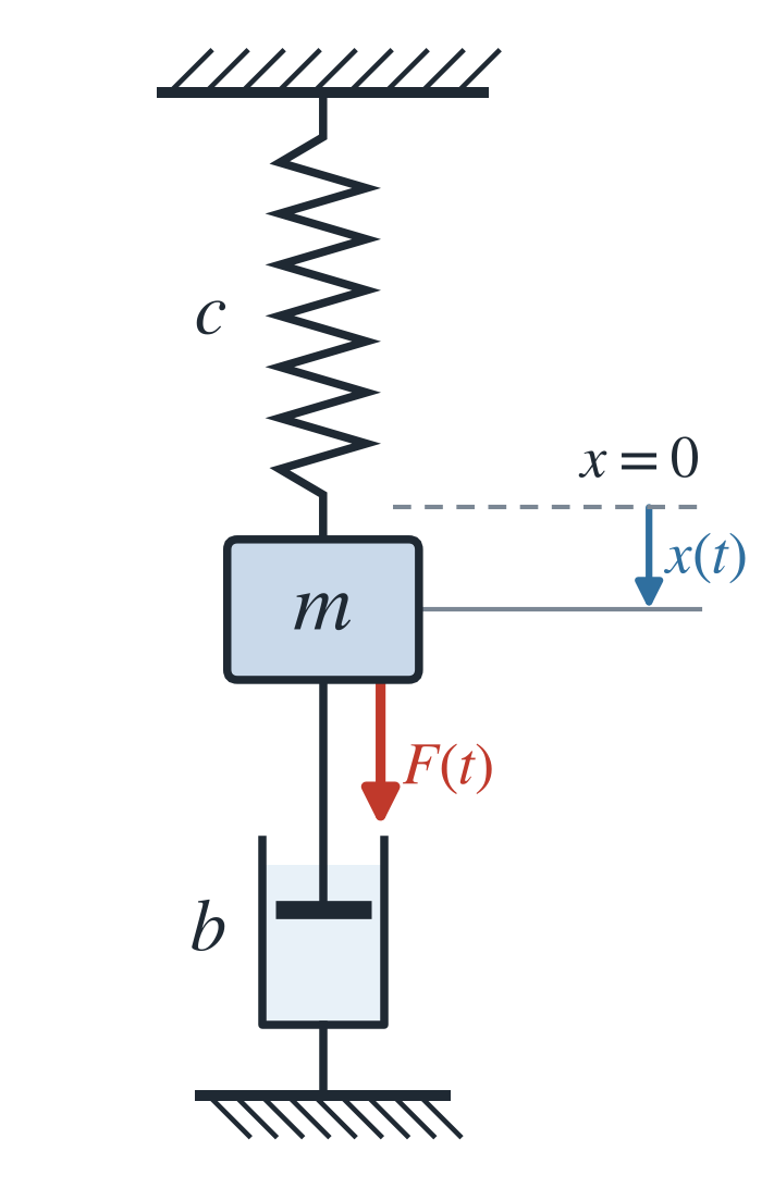
Three forces act on the mass:
- By Hooke’s law, the restoring force of the spring is \[ F_1 = -c\,x(t). \]
- According to experience, the damping force is proportional to the velocity and always opposes the motion: \[ F_2 = -b v = -b \dot{x}(t). \]
- In addition, there is an externally applied force, e.g., via an eccentric: \[ F_3 = F(t). \]
Further forces such as gravity or the inertial force are neglected. By Newton’s second law, \[ m\ddot{x} = F_1 + F_2 + F_3, \] from which (taking friction into account) the second-order ODE \[ m \ddot{x} = -cx - b \dot{x} + F(t) \quad \text{or} \quad m \ddot{x} + b\dot{x} + cx = F(t) \] follows. The motion of a mass-spring oscillator is thus described by a linear second-order ODE with constant coefficients. Depending on whether an external force and damping are present, we distinguish in the following the free undamped, the free damped, and the forced oscillation. If the damping is too strong, the system no longer oscillates but returns aperiodically to the rest position (overdamped case, Section 2.7.4). Definition 2.10 summarizes the oscillation types (Papula 2015, sec. IV.4.1.1).
Definition 2.10 (Differential Equation of a Mechanical Oscillation (Oscillation Equation)) The motion of a mass-spring oscillator (Definition 2.9) is described by the linear second-order ODE with constant coefficients \[ m \ddot{x} + b \dot{x} + c x = F(t) \tag{2.7}\] It is called the oscillation equation. Here, \(m\) is the mass, \(b\) the damper constant, \(c\) the spring constant, and \(F(t)\) the time-dependent external force acting on the system.
Three special types of oscillation are distinguished:
- Free undamped oscillation: Neither an external force nor damping acts on the system, i.e., \(F(t) \equiv 0\) and \(b = 0\): \[ m \ddot{x} + c x = 0. \]
- Free damped oscillation: No external force acts on the system, but it is damped, i.e., \(F(t) \equiv 0\) and \(b \neq 0\): \[ m \ddot{x} + b \dot{x} + c x = 0. \]
- Forced oscillation: A time-dependent periodic force \(F(t) = F_0 \sin(\omega t)\) with the excitation angular frequency \(\omega\) acts on the system: \[ m \ddot{x} + b \dot{x} + c x = F_0 \sin(\omega t). \]
2.7.2 Free Undamped Oscillation
In what follows, we need the addition theorems for sine and cosine as well as the representation of a linear combination of sine and cosine as a phase-shifted sine oscillation.
Theorem 2.8 (Addition Theorem for the Sine) \[ \sin(x+y) = \sin(x)\cos(y) + \cos(x)\sin(y) \]
Lemma 2.1 (Phase-Shifted Sine Oscillation) For \(C_1, C_2 \in \mathbb{R}\), not both zero, \[ C_1 \sin(x) + C_2 \cos(x) = A \sin(x + \varphi) \] holds with the amplitude \[ A = \sqrt{C_1^2 + C_2^2} \] and the phase angle \(\varphi\), which is uniquely determined up to multiples of \(2\pi\) by \[ \cos(\varphi) = \frac{C_1}{A} \quad \text{and} \quad \sin(\varphi) = \frac{C_2}{A}. \] Depending on the quadrant, \[ \varphi = \begin{cases} \arctan(C_2/C_1) & \text{for } C_1 > 0, \\ \arctan(C_2/C_1) + \pi & \text{for } C_1 < 0, \\ \pi/2 & \text{for } C_1 = 0,\ C_2 > 0, \\ -\pi/2 & \text{for } C_1 = 0,\ C_2 < 0. \end{cases} \]
Proof. Since \((C_1/A)^2 + (C_2/A)^2 = 1\), the point \((C_1/A, C_2/A)\) lies on the unit circle. Hence there is an angle \(\varphi\) with \(\cos(\varphi) = C_1/A\) and \(\sin(\varphi) = C_2/A\), and it is unique up to multiples of \(2\pi\). The addition theorem for the sine yields \[\begin{align*} A \sin(x + \varphi) &= A \sin(x)\cos(\varphi) + A \cos(x)\sin(\varphi) \\ &= A \sin(x)\frac{C_1}{A} + A \cos(x)\frac{C_2}{A} \\ &= C_1 \sin(x) + C_2 \cos(x). \end{align*}\] For \(C_1 \neq 0\), \(\tan(\varphi) = C_2/C_1\). The arctangent returns only angles between \(-\pi/2\) and \(\pi/2\), that is, in the first or fourth quadrant, where \(\cos(\varphi) > 0\). For \(C_1 > 0\), this is the angle sought. For \(C_1 < 0\), \(\cos(\varphi) < 0\) and the angle sought is shifted by \(\pi\). This shift leaves \(\tan(\varphi)\) unchanged but reverses the signs of sine and cosine. For \(C_1 = 0\), \(\cos(\varphi) = 0\) and \(\sin(\varphi) = C_2/|C_2| = \pm 1\), so \(\varphi = \pm\pi/2\).
Remark 2.3 (Computing the Phase Angle in Python). In Python, numpy.arctan2(C2, C1) computes the phase angle without a case distinction.
2.7.2.1 General Solution
Theorem 2.9 (General Solution of the Free Undamped Oscillation) In the simplest case, without damping and without external force, the ODE (equation of motion) of the spring pendulum reads \[ m \ddot{x} + cx = 0 \quad \text{or} \quad \ddot{x} + \omega_0^2 x = 0 \tag{2.8}\] with \(\omega_0^2 = c/m\).
The characteristic equation associated with Equation 2.8, \[ \lambda^2 + \omega_0^2 = 0 \] has the complex conjugate solutions \[ \lambda_{1,2} = \pm \mathrm{j} \omega_0. \] By Equation 2.5, the fundamental basis of the homogeneous ODE Equation 2.8 is then \[ y_1 = \sin(\omega_0 t) \quad \text{and} \quad y_2 = \cos(\omega_0 t), \] from which the general solution of the equation of motion follows: \[ x(t) = C_1 \sin(\omega_0 t) + C_2 \cos(\omega_0 t), \tag{2.9}\] with the angular frequency \(\omega_0 = \sqrt{c/m}\) and \(C_1, C_2 \in \mathbb{R}\).
Remark 2.4 (Alternative Representation of the Phase-Shifted Sine Oscillation). By Lemma 2.1, the general solution Equation 2.9 can also be represented as a phase-shifted sine oscillation \[ x(t) = A \sin(\omega_0 t + \varphi), \quad t \geq 0, \] with the amplitude \(A\) of the oscillation.
2.7.2.2 Interpretation of the General Solution
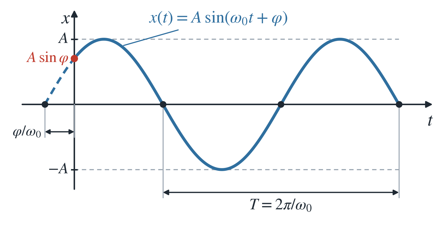
Lemma 2.2 (Period of the Oscillation) The system oscillates harmonically with the angular frequency \(\omega_0 = \sqrt{c/m}\), which is called the natural angular frequency (natural frequency for short). It has the period of oscillation \[ T = \frac{2\pi}{\omega_0} = 2\pi \sqrt{m/c}, \] see Figure 2.3.
Proof. \(x(t) = A \sin(\omega_0 t + \varphi)\) is periodic with the period \(T = 2\pi/\omega_0\) because \[ x(t + T) = A \sin(\omega_0 (t + T) + \varphi) = A \sin(\omega_0 t + 2\pi + \varphi) = A \sin(\omega_0 t + \varphi) = x(t). \]
The amplitude and the phase angle \(\varphi\) of the oscillation depend on the initial conditions \(x(0)\) and \(v(0)\).
2.7.2.3 Influence of the Spring Constant and the Mass on the Natural Angular Frequency
The natural angular frequency \(\omega_0 = \sqrt{c/m}\) depends only on the ratio of the spring constant \(c\) to the mass \(m\), not on the amplitude. The spring constant is not a force; it states how strongly the restoring force \(F_1 = -c\,x\) grows with the displacement. Writing the equation of motion Equation 2.8 in the form \[ \ddot{x} = -\frac{c}{m}\, x = -\omega_0^2\, x \] reveals the reason: for the same displacement \(x\), the acceleration of the mass toward the rest position is the larger, the larger \(c/m\) is. The mass then returns to the rest position more quickly, and the oscillation runs faster.
- Constant mass, modified spring constant. A stiffer spring (larger \(c\)) exerts a larger restoring force on the same mass at the same displacement. The natural angular frequency grows with the square root of the spring constant, and the period decreases accordingly: \[ \omega_0 \sim \sqrt{c}, \qquad T \sim \frac{1}{\sqrt{c}}. \] Quadrupling \(c\) doubles \(\omega_0\) and halves \(T\) (Figure 2.4). Accordingly, a softer spring makes the system oscillate more slowly.
- Constant spring constant, modified mass. A larger mass is more inert: the same restoring force gives it a smaller acceleration. The natural angular frequency decreases with the square root of the mass, and the period grows: \[ \omega_0 \sim \frac{1}{\sqrt{m}}, \qquad T \sim \sqrt{m}. \] Quadrupling \(m\) halves \(\omega_0\) and doubles \(T\) (Figure 2.5). Accordingly, a lighter mass oscillates faster.
In general, the natural angular frequency changes by the factor \(\sqrt{k}\) when \(c\) is multiplied by the factor \(k\), and by the factor \(1/\sqrt{k}\) when \(m\) is multiplied by \(k\). If \(c\) and \(m\) change by the same factor, \(\omega_0\) remains unchanged. For example, \(m = 1\,\mathrm{kg}\) and \(c = 4\,\mathrm{N/m}\) give \(\omega_0 = 2\,\mathrm{s}^{-1}\) and \(T = \pi\,\mathrm{s} \approx 3.14\,\mathrm{s}\). With \(c = 16\,\mathrm{N/m}\), one obtains \(\omega_0 = 4\,\mathrm{s}^{-1}\) and \(T \approx 1.57\,\mathrm{s}\); with \(m = 4\,\mathrm{kg}\) and \(c = 4\,\mathrm{N/m}\), by contrast, \(\omega_0 = 1\,\mathrm{s}^{-1}\) and \(T \approx 6.28\,\mathrm{s}\).
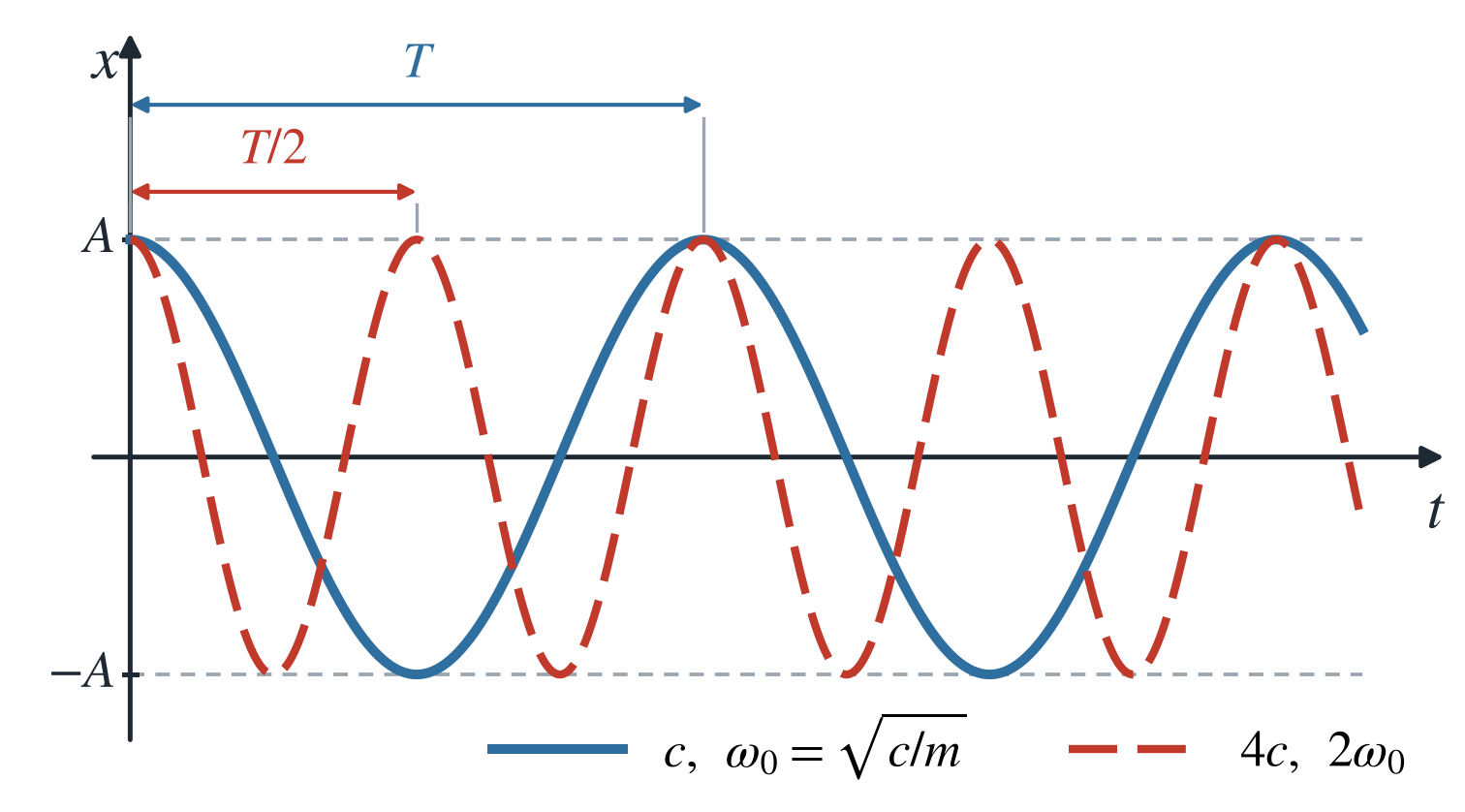
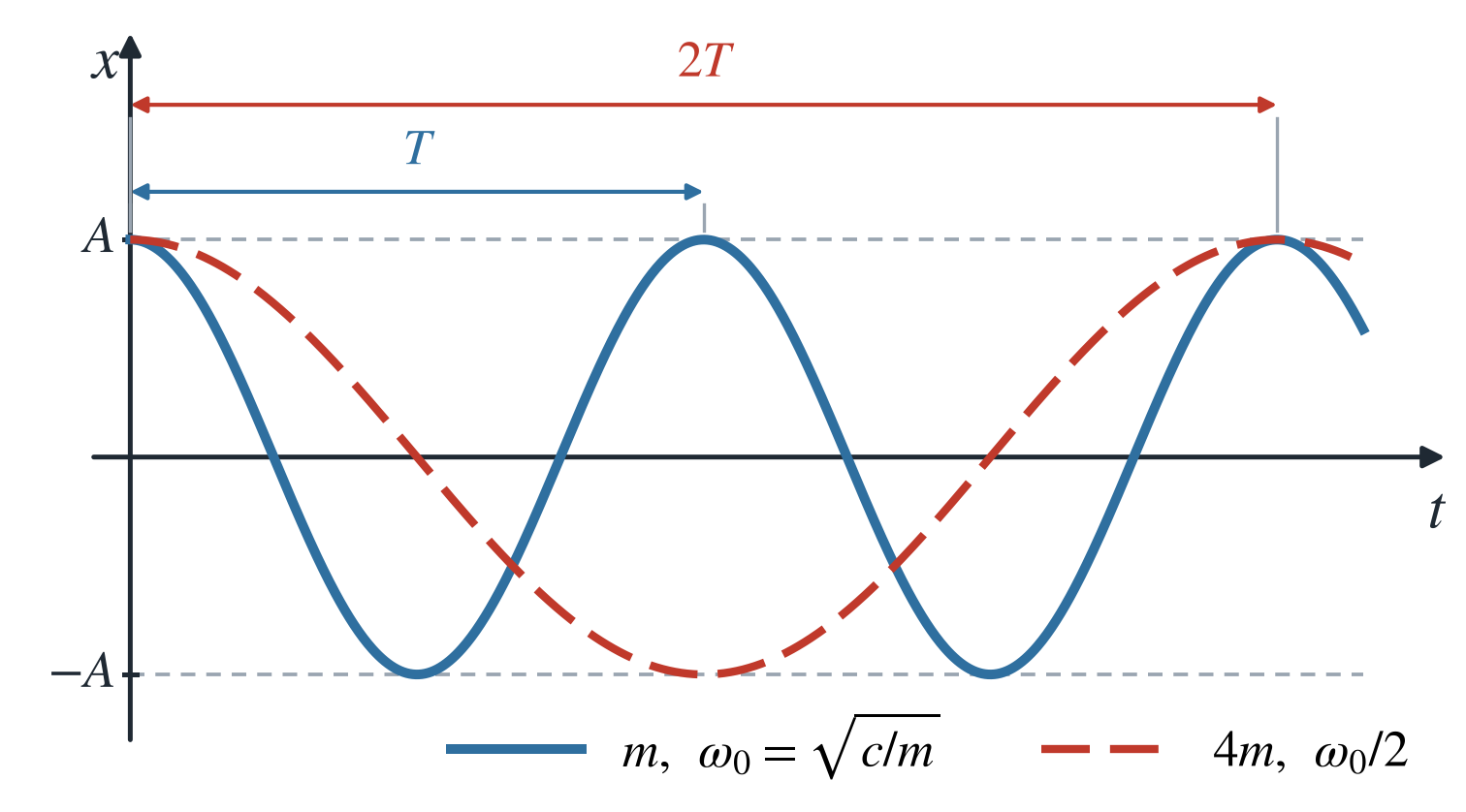
Both dependencies can be explored in the following animation by changing the spring constant \(c\) at fixed \(m\) or the mass \(m\) at fixed \(c\).
The animation at https://advm1.gm.fh-koeln.de/~bartz/bart26y/ shows Figure 2.3 and the mass-spring oscillator from Figure 2.2 (without external force) side by side. The point on the curve \(x(t)\) and the mass move in sync. The mass \(m\), the spring constant \(c\), and the initial conditions \(x(0)\) and \(v(0)\) can be adjusted; the amplitude \(A\), the phase angle \(\varphi\), and the period \(T\) adapt accordingly. For an easier visualization, the animation shows the displacement as positive upward, so that the mass and the point on the curve are at the same height; the checkbox “x positive downward” sets the direction of Figure 2.2. The equation of motion does not change.
Example 2.34 (Undamped Oscillation Starting from Rest) Let the system start from rest with the displacement \(x_0\) and the velocity \(v_0 = 0\). With the derivative of Equation 2.9, \[ \dot{x}(t) = C_1 \omega_0 \cos(\omega_0 t) - C_2 \omega_0 \sin(\omega_0 t), \] the conditions \(x(0) = x_0\) and \(\dot{x}(0) = 0\) yield the values \[ C_1 = 0 \quad \text{and} \quad C_2 = x_0. \] Substituting into the general solution Equation 2.9 yields the particular solution \[ x(t) = x_0 \cos(\omega_0 t), \] where \(x_0\) is the displacement of the mass at time \(t = 0\). The mass-spring oscillator thus oscillates with the natural angular frequency \(\omega_0 = \sqrt{c/m}\) and the amplitude \(A = x_0\), see Figure 2.6.
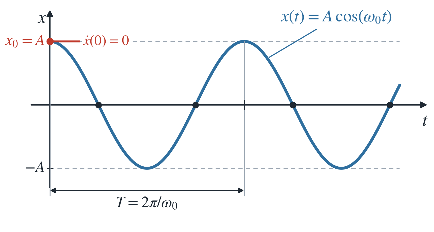
The following numerical example follows Papula (2015, sec. IV.4.1.2).
Example 2.35 (Free Undamped Oscillation) We investigate the motion of an oscillatory mechanical system with the mass \(m = 10\) kg and the spring constant \(c = 250\) N/m under the initial conditions \[ x(0) = 0.6\,\text{m} \quad \text{and} \quad v(0) = 0\,\text{m/s}. \] The natural angular frequency of the system is \[ \omega_0 = \sqrt{\frac{c}{m}} = \sqrt{\frac{250\,\text{N/m}}{10\,\text{kg}}} = 5\,\text{s}^{-1}. \] By Equation 2.9, the equation of motion \(\ddot{x} + 25x = 0\) has the general solution \[ x(t) = C_1 \sin(5t) + C_2 \cos(5t). \] We omit the units in the intermediate calculations. From \(x(0) = C_2 = 0.6\) and \(\dot{x}(0) = 5C_1 = 0\) it follows that \(C_1 = 0\) and \(C_2 = 0.6\). The system thus oscillates harmonically according to \[ x(t) = 0.6\,\text{m} \cdot \cos(5\,\text{s}^{-1} \cdot t), \quad t \geq 0. \] The period is \(T = 2\pi/\omega_0 = 0.4\pi\,\text{s} \approx 1.26\,\text{s}\), the amplitude \(A = 0.6\) m. This is the special case \(x_0 = 0.6\) m of Example 2.34.
What does the value \(\omega_0 = 5\,\text{s}^{-1}\) mean? The system neither performs five oscillations per second, nor does one oscillation take five seconds. The natural angular frequency states how fast the phase angle \(\omega_0 t\) in the argument of the cosine grows, here by \(5\) rad per second; the unit \(\text{s}^{-1}\) is to be read as rad/s. One full oscillation, i.e., the path from \(x = A\) via \(x = -A\) back to \(x = A\), corresponds to the phase angle \(2\pi \approx 6.28\) rad. For this, the system needs the period \(T = 2\pi/(5\,\text{s}^{-1}) \approx 1.26\) s, i.e., slightly more than one second. The number of full oscillations per second is the frequency \[ \nu_0 = \frac{\omega_0}{2\pi} = \frac{1}{T} = \frac{5}{2\pi}\,\text{s}^{-1} \approx 0.80\,\text{Hz}. \] In one second, the system thus performs about \(0.8\) full oscillations; five full oscillations take \(5T \approx 6.3\) s. Angular frequency and frequency differ by the factor \(2\pi\).
2.7.3 Free Damped Oscillation
In a free damped oscillation, a damping force acts on the mass in addition to the restoring force. The ODE of the spring pendulum then reads \[ m \ddot{x} + b \dot{x} + cx = 0 \] or \[ \ddot{x} + 2\delta \dot{x} + \omega_0^2 x = 0 \tag{2.10}\] with the damping factor \(\delta = b/(2m)\) and the natural angular frequency \(\omega_0 = \sqrt{c/m}\).
The associated characteristic equation \[ \lambda^2 + 2\delta \lambda + \omega_0^2 = 0 \tag{2.11}\] has the solutions \[ \lambda_{1,2} = -\delta \pm \sqrt{\delta^2 - \omega_0^2}, \] whose nature is decided by the discriminant \(\Delta = \delta^2 - \omega_0^2\):
- \(\Delta < 0\), i.e., \(\delta < \omega_0\): weakly damped oscillation,
- \(\Delta = 0\), i.e., \(\delta = \omega_0\): aperiodic limiting case (critically damped case),
- \(\Delta > 0\), i.e., \(\delta > \omega_0\): aperiodic motion (overdamped case).
Theorem 2.10 (General Solution of the Equation of Motion of a Free Damped Spring Pendulum) The solutions of Equation 2.10 belong to one of three types of oscillation:
Weakly damped oscillation (\(\delta < \omega_0\)): The characteristic equation has the complex conjugate solutions \[ \lambda_{1,2} = -\delta \pm \mathrm{j} \sqrt{\omega_0^2 - \delta^2} = -\delta \pm \mathrm{j} \omega_{\mathrm{d}}, \] where \(\omega_{\mathrm{d}} = \sqrt{\omega_0^2 - \delta^2}\) is the natural angular frequency of the damped system. The general solution is \[ x(t) = \mathrm{e}^{-\delta t} \left[ C_1 \sin(\omega_{\mathrm{d}} t) + C_2 \cos(\omega_{\mathrm{d}} t) \right] \] with \(C_1, C_2 \in \mathbb{R}\), or equivalently \[ x(t) = A_{\mathrm{d}} \mathrm{e}^{-\delta t} \sin(\omega_{\mathrm{d}} t + \varphi_{\mathrm{d}}) \] with the amplitude \(A_{\mathrm{d}} > 0\) and the phase angle \(0 \leq \varphi_{\mathrm{d}} \leq 2\pi\).
Aperiodic limiting case (\(\delta = \omega_0\)): The characteristic equation has the double real solution \(\lambda_{1,2} = -\delta\). The general solution is \[ x(t) = \left[ C_1 t + C_2 \right] \mathrm{e}^{-\delta t} \tag{2.12}\] with \(C_1, C_2 \in \mathbb{R}\).
Aperiodic motion under strong damping (overdamped case, \(\delta > \omega_0\)): The characteristic equation has two distinct real negative solutions \(\lambda_1\) and \(\lambda_2\). The general solution is \[ x(t) = C_1 \mathrm{e}^{\lambda_1 t} + C_2 \mathrm{e}^{\lambda_2 t} \] with \(C_1, C_2 \in \mathbb{R}\).
Proof. The three cases follow from Proposition 2.2 with \(a = 2\delta\), \(b = \omega_0^2\), and \(\lambda_{1,2} = -\delta \pm \sqrt{\Delta}\). The representation with \(A_{\mathrm{d}}\) and \(\varphi_{\mathrm{d}}\) follows from the sine addition theorem with \(C_1 = A_{\mathrm{d}} \cos\varphi_{\mathrm{d}}\) and \(C_2 = A_{\mathrm{d}} \sin\varphi_{\mathrm{d}}\).
2.7.3.1 Weak Damping (Underdamped Case)
Theorem 2.11 (General Solution of the Equation of Motion of a Free Damped Spring Pendulum under Weak Damping) Under weak damping, \(\Delta = \delta^2 - \omega_0^2 < 0\), i.e., \(\delta < \omega_0\). With the abbreviation \[ \omega_{\mathrm{d}}^2 = \omega_0^2 - \delta^2 > 0 \] the characteristic equation Equation 2.11 has the complex conjugate solutions \[ \lambda_{1,2} = -\delta \pm \sqrt{\delta^2 - \omega_0^2} = -\delta \pm \sqrt{- (\omega_0^2 - \delta^2)} = -\delta \pm \sqrt{- \omega_{\mathrm{d}}^2} = -\delta \pm \mathrm{j} \omega_{\mathrm{d}}. \] By Equation 2.5 with \(\alpha = -\delta\) and \(\omega = \omega_{\mathrm{d}}\), the general solution stated in Theorem 2.10 follows: \[ x(t) = A_{\mathrm{d}} \mathrm{e}^{-\delta t} \sin(\omega_{\mathrm{d}} t + \varphi_{\mathrm{d}}). \tag{2.13}\]
This is a damped oscillation whose natural angular frequency is reduced compared with the undamped oscillation, \[ \omega_{\mathrm{d}} = \sqrt{\omega_0^2 - \delta^2} < \omega_0, \] see Figure 2.7.
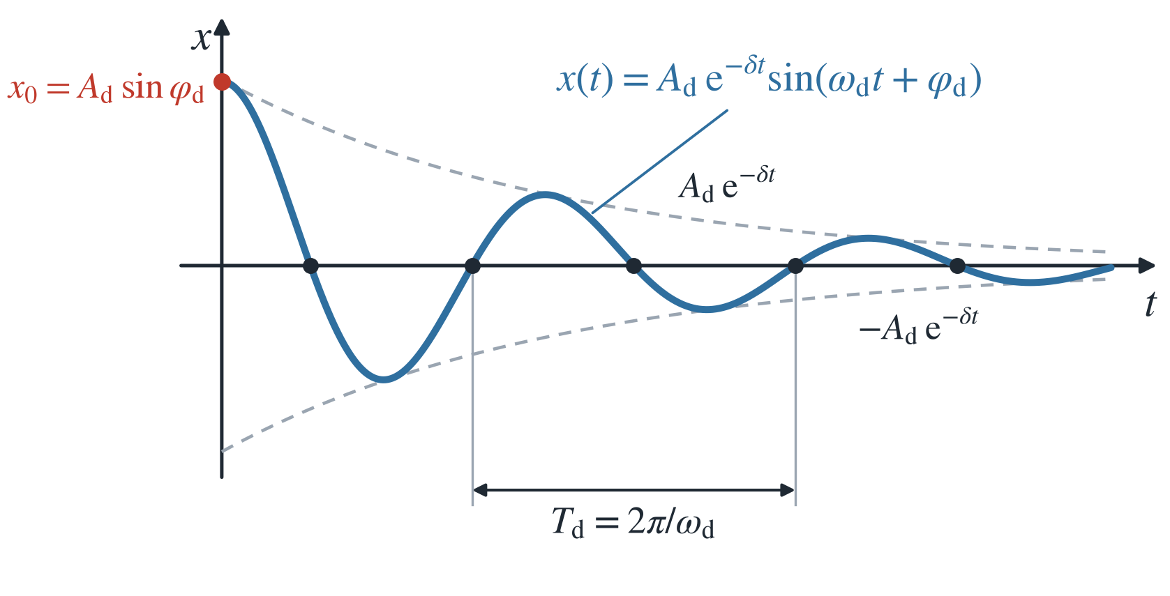
Example 2.36 (Weakly Damped Oscillation Starting from Rest) Consider the free damped oscillation Equation 2.10, \[ m \ddot{x} + b \dot{x} + cx = 0 \qquad \text{or} \qquad \ddot{x} + 2\delta \dot{x} + \omega_0^2 x = 0, \] with the damping factor \(\delta = b/(2m) > 0\) and the natural angular frequency \(\omega_0 = \sqrt{c/m}\) of the undamped system. Let the system be weakly damped (\(\delta < \omega_0\)) and start from rest at time \(t = 0\) with the displacement \(x_0 = A > 0\) and the velocity \(v_0 = 0\). We seek the amplitude \(A_{\mathrm{d}}\) and the phase angle \(\varphi_{\mathrm{d}}\) of the particular solution.
Approach. The starting point is the general solution for weak damping (case 1 in Theorem 2.10, see Section 2.7.3.1) \[ x(t) = A_{\mathrm{d}} \mathrm{e}^{-\delta t} \sin(\omega_{\mathrm{d}} t + \varphi_{\mathrm{d}}), \qquad \omega_{\mathrm{d}} = \sqrt{\omega_0^2 - \delta^2} > 0, \] with \(A_{\mathrm{d}} > 0\). The two parameters are determined from the initial conditions.
Step 1: Velocity. By the product rule, \[ \dot{x}(t) = -\delta A_{\mathrm{d}} \mathrm{e}^{-\delta t} \sin(\omega_{\mathrm{d}} t + \varphi_{\mathrm{d}}) + \omega_{\mathrm{d}} A_{\mathrm{d}} \mathrm{e}^{-\delta t} \cos(\omega_{\mathrm{d}} t + \varphi_{\mathrm{d}}) = A_{\mathrm{d}} \mathrm{e}^{-\delta t} \left[ \omega_{\mathrm{d}} \cos(\omega_{\mathrm{d}} t + \varphi_{\mathrm{d}}) - \delta \sin(\omega_{\mathrm{d}} t + \varphi_{\mathrm{d}}) \right]. \]
Step 2: Initial conditions. For \(t = 0\), \(\mathrm{e}^{0} = 1\), so \[ x(0) = A_{\mathrm{d}} \sin \varphi_{\mathrm{d}} = A, \] \[ \dot{x}(0) = A_{\mathrm{d}} \left( \omega_{\mathrm{d}} \cos \varphi_{\mathrm{d}} - \delta \sin \varphi_{\mathrm{d}} \right) = 0. \]
Step 3: Phase angle. Since \(A_{\mathrm{d}} \neq 0\), the second equation yields \[ \omega_{\mathrm{d}} \cos \varphi_{\mathrm{d}} = \delta \sin \varphi_{\mathrm{d}}. \] The first equation yields \(\sin \varphi_{\mathrm{d}} = A/A_{\mathrm{d}} > 0\), so \(\delta > 0\) and \(\omega_{\mathrm{d}} > 0\) imply \(\cos \varphi_{\mathrm{d}} > 0\) as well. The angle therefore lies in the first quadrant, \(0 < \varphi_{\mathrm{d}} < \pi/2\), and division by \(\delta \cos \varphi_{\mathrm{d}}\) gives \[ \tan \varphi_{\mathrm{d}} = \frac{\omega_{\mathrm{d}}}{\delta} \qquad \Longrightarrow \qquad \varphi_{\mathrm{d}} = \arctan\left(\frac{\omega_{\mathrm{d}}}{\delta}\right). \] The principal value of the arctangent is the correct choice here because for positive arguments it also lies between \(0\) and \(\pi/2\).
Step 4: Sine of the phase angle. For \(0 < \varphi_{\mathrm{d}} < \pi/2\), \(\sin \varphi_{\mathrm{d}} = \tan \varphi_{\mathrm{d}} / \sqrt{1 + \tan^2 \varphi_{\mathrm{d}}}\). With \(\delta^2 + \omega_{\mathrm{d}}^2 = \delta^2 + \omega_0^2 - \delta^2 = \omega_0^2\), it follows that \[ \sin \varphi_{\mathrm{d}} = \frac{\omega_{\mathrm{d}}/\delta}{\sqrt{1 + \omega_{\mathrm{d}}^2/\delta^2}} = \frac{\omega_{\mathrm{d}}}{\sqrt{\delta^2 + \omega_{\mathrm{d}}^2}} = \frac{\omega_{\mathrm{d}}}{\omega_0} \qquad \text{and likewise} \qquad \cos \varphi_{\mathrm{d}} = \frac{\delta}{\omega_0}. \]
Step 5: Amplitude. Substituting into the first initial condition \(A_{\mathrm{d}} \sin \varphi_{\mathrm{d}} = A\) yields \[ A_{\mathrm{d}} = \frac{A}{\sin \varphi_{\mathrm{d}}} = \frac{\omega_0}{\omega_{\mathrm{d}}} A. \]
Check. With the results of Steps 4 and 5, \[ x(0) = \frac{\omega_0}{\omega_{\mathrm{d}}} A \cdot \frac{\omega_{\mathrm{d}}}{\omega_0} = A \qquad \text{and} \qquad \dot{x}(0) = \frac{\omega_0}{\omega_{\mathrm{d}}} A \left( \omega_{\mathrm{d}} \frac{\delta}{\omega_0} - \delta \frac{\omega_{\mathrm{d}}}{\omega_0} \right) = 0. \]
Result. The particular solution is \[ x(t) = A_{\mathrm{d}} \mathrm{e}^{-\delta t} \sin(\omega_{\mathrm{d}} t + \varphi_{\mathrm{d}}) \] with the parameters \[ A_{\mathrm{d}} = \frac{\omega_0}{\omega_{\mathrm{d}}}A \qquad \text{and} \qquad \varphi_{\mathrm{d}} = \arctan\left(\frac{\omega_{\mathrm{d}}}{\delta}\right). \]
The numerical examples on damped oscillation follow Papula (2015, sec. IV.4.1.3).
Example 2.37 (Weak Damping) Consider an oscillatory mechanical system with the mass \(m = 10\) kg, the damper constant \(b = 80\) kg/s, and the spring constant \(c = 250\) N/m. The initial conditions are \[ x(0) = 0.6\,\text{m} \quad \text{and} \quad v(0) = 0\,\text{m/s}. \] The damping factor and the natural angular frequency of the undamped system are \[ \delta = \frac{b}{2m} = \frac{80\,\text{kg/s}}{20\,\text{kg}} = 4\,\text{s}^{-1} \quad \text{and} \quad \omega_0 = \sqrt{\frac{c}{m}} = 5\,\text{s}^{-1}. \] The equation of motion (without units) is therefore \(\ddot{x} + 8\dot{x} + 25x = 0\). Since \(\delta < \omega_0\), the system is weakly damped and oscillates with the natural angular frequency \[ \omega_{\mathrm{d}} = \sqrt{\omega_0^2 - \delta^2} = \sqrt{25 - 16}\,\text{s}^{-1} = 3\,\text{s}^{-1}. \]
The general solution of the ODE is therefore \[ x(t) = \mathrm{e}^{-4t} \left[ C_1 \sin(3t) + C_2 \cos(3t) \right] \] or, in the form of a phase-shifted sine oscillation, \[ x(t) = A_{\mathrm{d}} \mathrm{e}^{-4t} \sin(3t + \varphi_{\mathrm{d}}). \tag{2.14}\]
We consider two ways of solving:
- First, the solution using the formulas from Example 2.36: By Example 2.36 with \(A = 0.6\) m, the amplitude and the phase angle are \[ A_{\mathrm{d}} = \frac{\omega_0}{\omega_{\mathrm{d}}} A = \frac{5}{3} \cdot 0.6\,\text{m} = 1\,\text{m} \quad \text{and} \quad \varphi_{\mathrm{d}} = \arctan\left( \frac{\omega_{\mathrm{d}}}{\delta} \right) = \arctan\left( \frac{3}{4} \right) \approx 0.6435. \] The system therefore performs the damped oscillation \[ x(t) = 1\,\text{m} \cdot \mathrm{e}^{-4\,\text{s}^{-1} t} \sin(3\,\text{s}^{-1} \cdot t + 0.6435), \quad t \geq 0. \]
- Alternatively, we substitute the initial conditions directly into Equation 2.14. With the derivative \[ \dot{x}(t) = A_{\mathrm{d}} \mathrm{e}^{-4t} \left[ 3 \cos(3t + \varphi_{\mathrm{d}}) - 4 \sin(3t + \varphi_{\mathrm{d}}) \right] \] we obtain (without units) the system of equations \[ \begin{aligned} \text{I:} \quad & x(0) = A_{\mathrm{d}} \sin \varphi_{\mathrm{d}} = 0.6, \\ \text{II:} \quad & \dot{x}(0) = A_{\mathrm{d}} \left( 3 \cos \varphi_{\mathrm{d}} - 4 \sin \varphi_{\mathrm{d}} \right) = 0. \end{aligned} \] Since \(A_{\mathrm{d}} \neq 0\), II yields \[ 4 \sin \varphi_{\mathrm{d}} = 3 \cos \varphi_{\mathrm{d}} \Rightarrow \tan \varphi_{\mathrm{d}} = \frac{3}{4} \Rightarrow \varphi_{\mathrm{d}} = \arctan\left( \frac{3}{4} \right) \approx 0.6435. \] With \(\sin \varphi_{\mathrm{d}} = 3/5\) (cf. \(\sin \varphi_{\mathrm{d}} = \omega_{\mathrm{d}}/\omega_0\) in Example 2.36), I yields \[ A_{\mathrm{d}} = \frac{0.6\,\text{m}}{\sin \varphi_{\mathrm{d}}} = \frac{0.6\,\text{m}}{3/5} = 1\,\text{m}. \]
2.7.4 Strong Damping (Aperiodic Behavior, Overdamped Case)
Theorem 2.12 (General Solution of the Equation of Motion of a Free Damped Spring Pendulum under Strong Damping) Under strong damping, \(\Delta = \delta^2 - \omega_0^2 > 0\), i.e., \(\delta > \omega_0\). The characteristic equation Equation 2.11 then has the two distinct real solutions \[ \lambda_1 = -\delta + \sqrt{\delta^2 - \omega_0^2} < 0 \quad \text{and} \quad \lambda_2 = -\delta - \sqrt{\delta^2 - \omega_0^2} < 0, \] i.e., \(\lambda_2 < \lambda_1 < 0\). The general solution of the ODE Equation 2.10 is a linear combination of two monotonically decreasing exponential functions, \[ x(t) = C_1 \mathrm{e}^{\lambda_1 t} + C_2 \mathrm{e}^{\lambda_2 t}, \quad C_1, C_2 \in \mathbb{R}. \tag{2.15}\] The mechanical system no longer oscillates but approaches the equilibrium state asymptotically, see Figure 2.8.
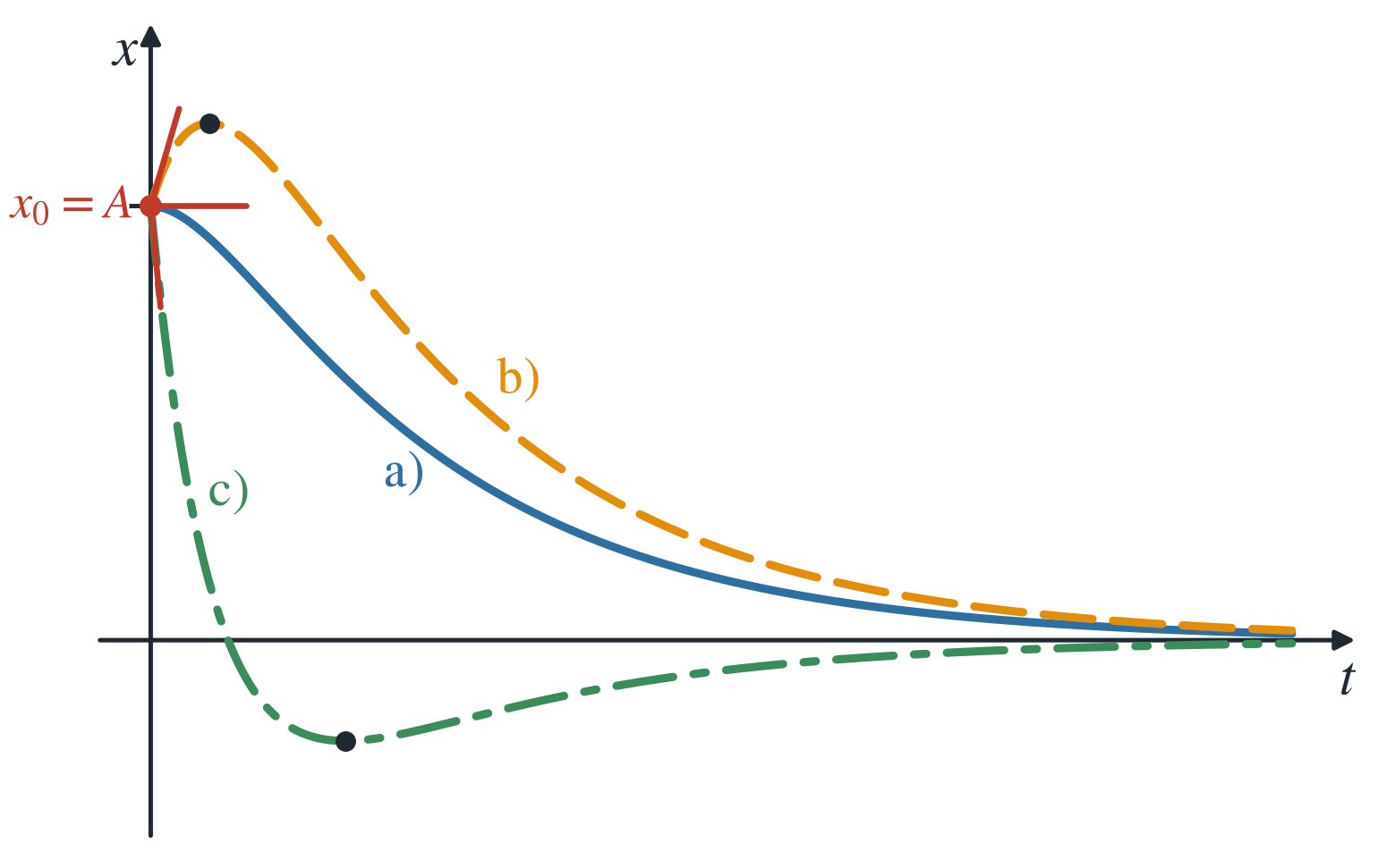
Example 2.38 (Overdamped Case: Motion Starting from Rest) If the system starts from rest, the initial conditions are \(x(0) = A\) and \(v(0) = 0\). For the coefficients of the general solution Equation 2.15, \(x(0) = A\) and \(\dot{x}(0) = 0\) yield the linear system of equations \[\begin{align*} C_1 + C_2 &= A, \\ \lambda_1 C_1 + \lambda_2 C_2 &= 0 \end{align*}\] with the solutions \[ C_1 = \frac{\lambda_2}{\lambda_2 - \lambda_1} A \quad \text{and} \quad C_2 = \frac{\lambda_1}{\lambda_1 - \lambda_2} A. \] The particular solution is therefore \[ x(t) = \frac{\lambda_2}{\lambda_2 - \lambda_1} A \mathrm{e}^{\lambda_1 t} + \frac{\lambda_1}{\lambda_1 - \lambda_2} A \mathrm{e}^{\lambda_2 t}, \] see Figure 2.9.
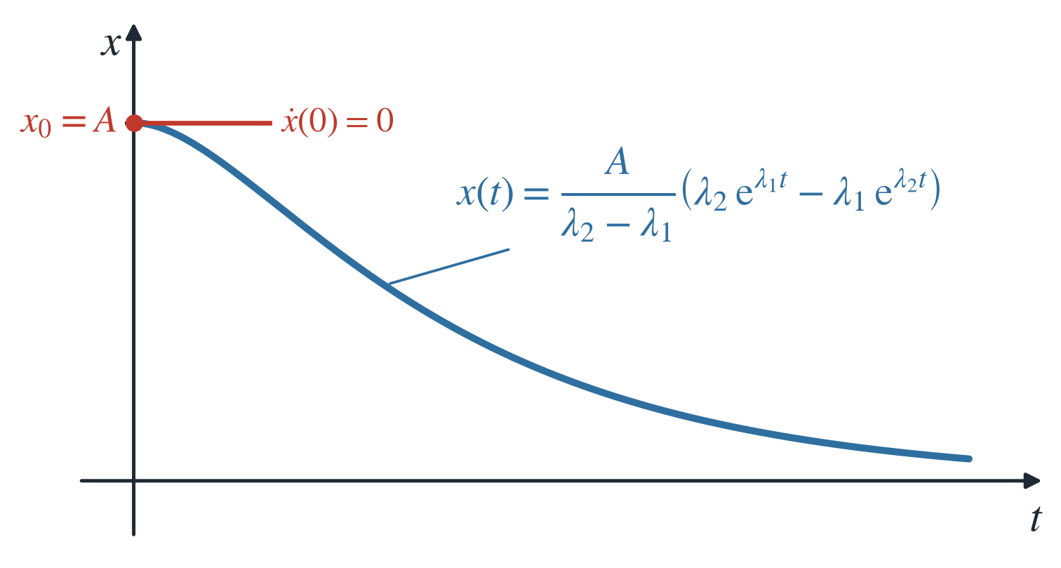
Example 2.39 (Overdamped Case: Motion Starting from the Equilibrium Position) If the system starts from the equilibrium position with the velocity \(v_0 > 0\), the initial conditions are \(x(0) = 0\) and \(v(0) = v_0\). From \[ x(0) = C_1 + C_2 = 0 \quad \text{and} \quad \dot{x}(0) = \lambda_1 C_1 + \lambda_2 C_2 = v_0 \] we obtain the coefficients \[ C_1 = \frac{v_0}{\lambda_1 - \lambda_2} \quad \text{and} \quad C_2 = - \frac{v_0}{\lambda_1 - \lambda_2} \] and hence the particular solution \[ x(t) = \frac{v_0}{\lambda_1 - \lambda_2} \left( \mathrm{e}^{\lambda_1 t} - \mathrm{e}^{\lambda_2 t} \right), \] see Figure 2.10.
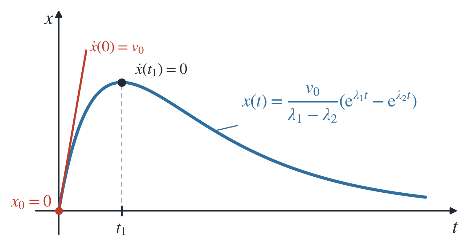
Example 2.40 (Strong Damping) Consider the equation of motion \[ \ddot{x} + 6 \dot{x} + 8.75\, x = 0 \] with the initial values \(x(0) = 0\) and \(v(0) = 8\). The characteristic equation has two distinct negative solutions: \[ \lambda^2 + 6\lambda + 8.75 = 0 \Rightarrow \lambda_1 = -2.5, \quad \lambda_2 = -3.5. \] The general solution is therefore \[ x(t) = C_1 \mathrm{e}^{-2.5\, t} + C_2 \mathrm{e}^{-3.5\, t}. \] From \(x(0) = C_1 + C_2 = 0\) it follows that \(C_2 = -C_1\). With \(\dot{x}(0) = -2.5\, C_1 - 3.5\, C_2 = 8\) we obtain \(-2.5\, C_1 + 3.5\, C_1 = C_1 = 8\), so \(C_1 = 8\) and \(C_2 = -8\). The particular solution is \[ x(t) = 8 \left( \mathrm{e}^{-2.5\, t} - \mathrm{e}^{-3.5\, t} \right), \quad t \geq 0. \] It is the special case \(v_0 = 8\) of Example 2.39 and describes an aperiodic motion (overdamped case) with the turning point at \[ t_1 = \frac{\ln(\lambda_2/\lambda_1)}{\lambda_1 - \lambda_2} = \ln(1.4) \approx 0.34, \] see Figure 2.10.
2.7.5 Aperiodic Limiting Case
2.7.5.1 General Solution of the Equation of Motion in the Aperiodic Limiting Case
For \(\Delta = \delta^2 - \omega_0^2 = 0\) we have the aperiodic limiting case. It separates the oscillations from the aperiodic motions. What is separated are the values of the damping factor \(\delta = b/(2m)\): at a fixed natural angular frequency \(\omega_0\), they fall into two ranges with fundamentally different motion:
- For \(\delta < \omega_0\) (weak damping, Section 2.7.3.1), the system oscillates. The mass swings about the rest position with the angular frequency \(\omega_{\mathrm{d}} = \sqrt{\omega_0^2 - \delta^2}\), passes through it infinitely often, and comes to rest with exponentially decreasing amplitude. The special case \(\delta = 0\) is the free undamped oscillation (Section 2.7.2).
- For \(\delta > \omega_0\) (strong damping, overdamped case, Section 2.7.4), the system does not oscillate. The mass creeps back to the rest position and passes through it at most once.
The aperiodic limiting case \(\delta = \omega_0\) lies exactly on the boundary between these ranges. It belongs to the aperiodic motions itself: as in the overdamped case, the mass passes through the rest position at most once (Figure 2.11). If the damping is increased starting from \(\delta = 0\), \(\omega_{\mathrm{d}}\) becomes smaller and smaller and the period \(T_{\mathrm{d}} = 2\pi/\omega_{\mathrm{d}}\) larger and larger. For \(\delta \to \omega_0\), \(\omega_{\mathrm{d}} \to 0\) and \(T_{\mathrm{d}} \to \infty\): a full oscillation would never be completed. The limiting case is thus the smallest damping at which the system no longer oscillates. For the damper constant, \(\delta = \omega_0\) means that \[ b = 2\sqrt{c\,m}. \] If the mass is released from rest, it returns to the rest position faster in the limiting case than with any stronger damping, without overshooting the rest position as with weaker damping.
| Case | Condition | Solutions of the characteristic equation | Motion | Section |
|---|---|---|---|---|
| undamped | \(\delta = 0\) | \(\lambda_{1,2} = \pm\mathrm{j}\omega_0\) | harmonic oscillation with constant amplitude | Section 2.7.2 |
| weak damping | \(0 < \delta < \omega_0\) | \(\lambda_{1,2} = -\delta \pm \mathrm{j}\omega_{\mathrm{d}}\) | damped oscillation, infinitely many zero crossings | Section 2.7.3.1 |
| aperiodic limiting case | \(\delta = \omega_0\) | \(\lambda_{1,2} = -\delta\) (double) | aperiodic, at most one zero crossing | Section 2.7.5 |
| strong damping (overdamped case) | \(\delta > \omega_0\) | \(\lambda_{1,2} = -\delta \pm \sqrt{\delta^2 - \omega_0^2}\) (real, distinct) | aperiodic, at most one zero crossing | Section 2.7.4 |
In the limiting case, the characteristic equation (Equation 2.11) has the double negative real solution \[ \lambda_{1,2} = -\delta. \] By Equation 2.4, the general solution of the ODE Equation 2.10 is the function given in Equation 2.12,
\[ x(t) = \left[ C_1 t + C_2 \right] \mathrm{e}^{-\delta t}, \quad C_1, C_2 \in \mathbb{R}. \tag{2.16}\]
The oscillatory mechanical system behaves similarly to the overdamped case. It moves aperiodically out of its initial position and approaches the equilibrium state asymptotically, see Figure 2.11.
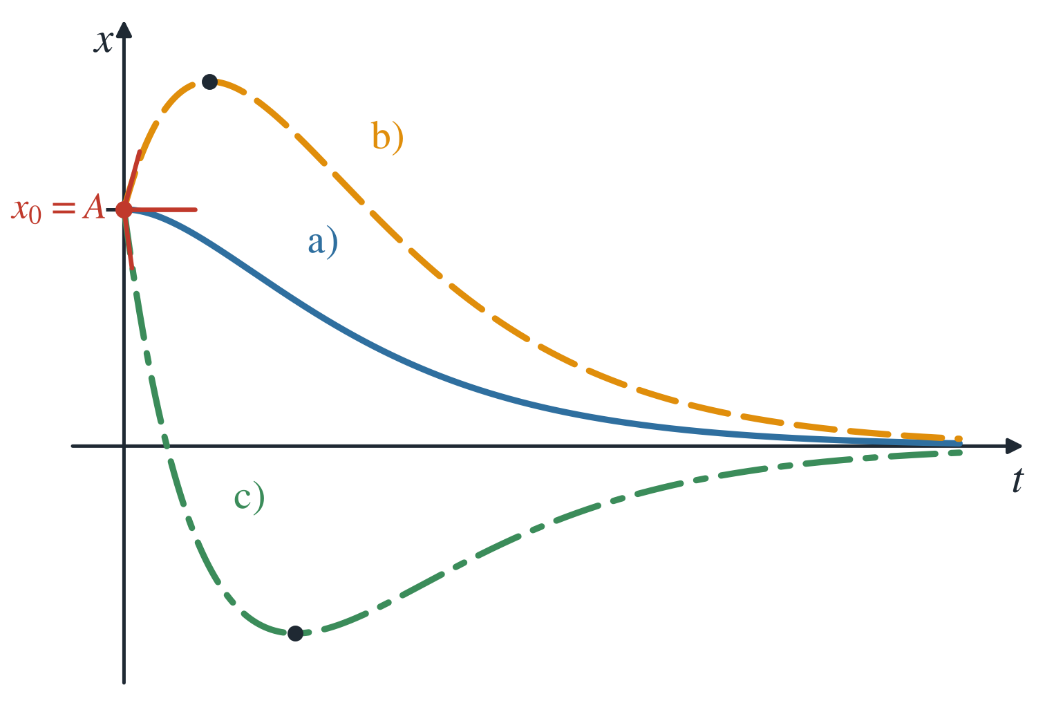
2.7.5.2 Special Cases of the Aperiodic Limiting Case
Example 2.41 (Aperiodic Limiting Case: Motion Starting from Rest) If the system starts from rest, the initial conditions are \(x(0) = A\) and \(v(0) = 0\). For the constants of the general solution Equation 2.12, it follows that \[ x(0) = C_2 = A \quad \text{and} \quad \dot{x}(0) = C_1 - \delta C_2 = 0, \] i.e., \(C_1 = \delta A\) and \(C_2 = A\). The particular solution is \[ x(t) = \left[ \delta A t + A \right] \mathrm{e}^{-\delta t}, \quad t \geq 0. \] The system moves aperiodically out of rest and approaches the equilibrium state asymptotically, see Figure 2.12.
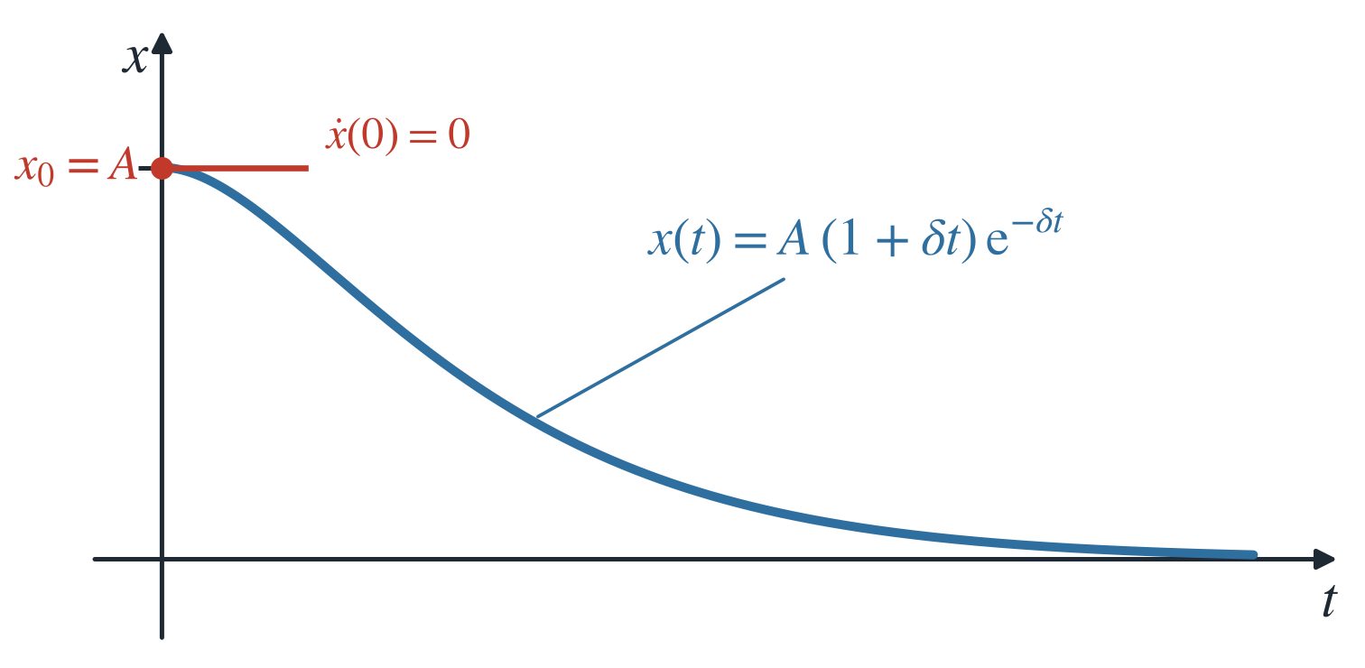
Example 2.42 (Aperiodic Limiting Case: Motion Starting from the Equilibrium Position) If the system, located in the equilibrium position, is set in motion at time \(t = 0\) with the velocity \(v_0 > 0\), the initial conditions are \(x(0) = 0\) and \(v(0) = v_0\).
With Equation 2.16 \[ x(t) = \left[ C_1 t + C_2 \right] \mathrm{e}^{-\delta t}, \quad C_1, C_2 \in \mathbb{R}. \] it follows from \[ x(0) = C_2 = 0 \quad \text{and} \quad \dot{x}(0) = C_1 - \delta C_2 = v_0 \] that \(C_1 = v_0\) and \(C_2 = 0\).
The particular solution is \[ x(t) = v_0\, t\, \mathrm{e}^{-\delta t}. \] Owing to the initial velocity, the mass first moves aperiodically out of the equilibrium position, reaches its turning point at time \(t_2 = 1/\delta\), and then approaches the equilibrium state asymptotically, see Figure 2.13.
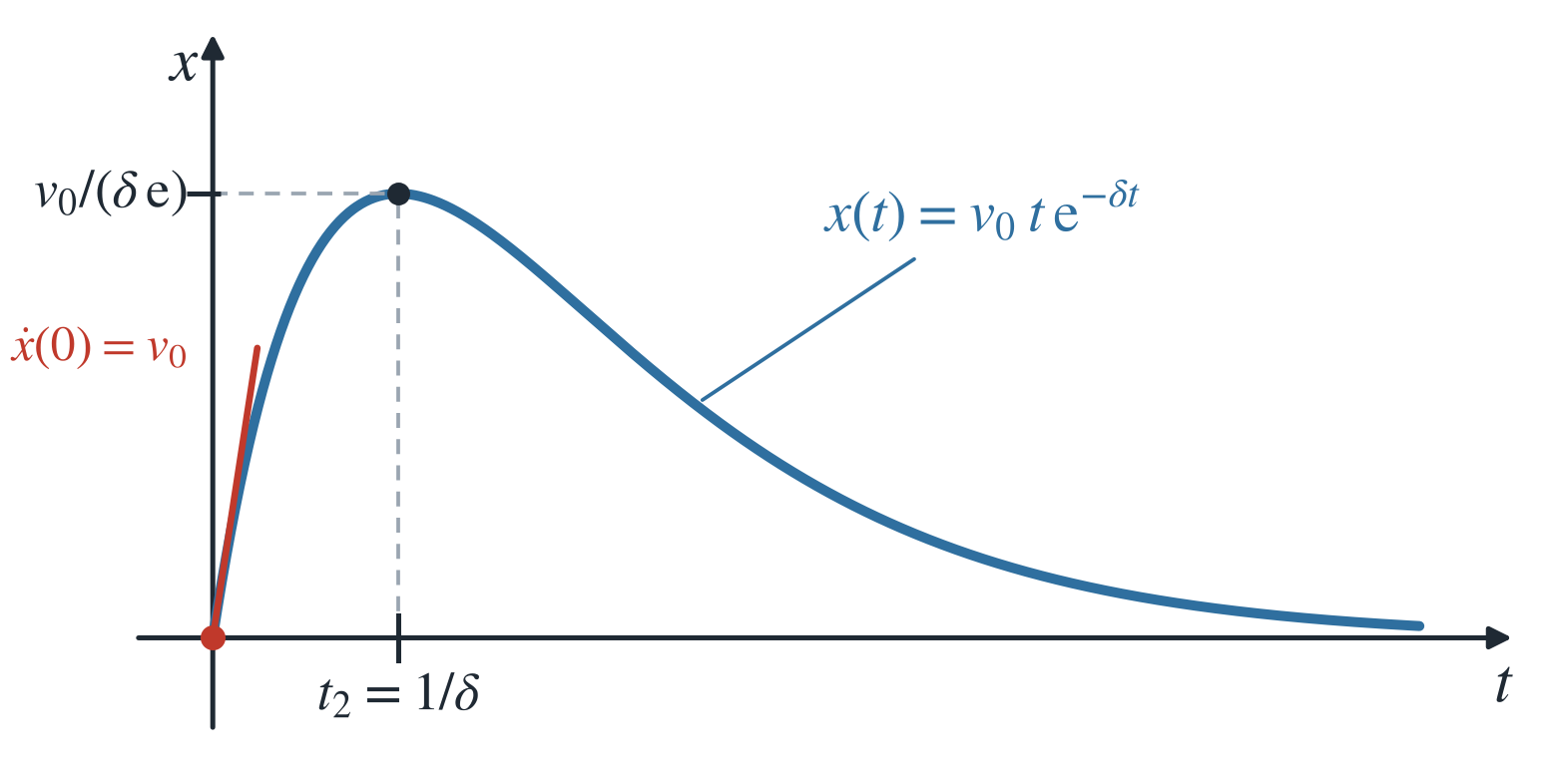
Example 2.43 (Aperiodic Limiting Case) Consider an oscillatory mechanical system with the spring constant \(c=200\) N/m and the damper constant \(b=60\) kg/s. How large must the oscillating mass \(m\) be for the aperiodic limiting case to occur?
The aperiodic limiting case occurs for \(\delta = \omega_0\), i.e., for \[ \frac{b}{2m} = \sqrt{\frac{c}{m}} \quad \text{or} \quad \frac{b^2}{4m^2} = \frac{c}{m}. \] Solving for \(m\) gives \[ m = \frac{b^2}{4c} = \frac{(60\,\text{kg/s})^2}{4 \cdot 200\,\text{N/m}} = 4.5\,\text{kg}. \] For \(m > 4.5\) kg, \(\delta < \omega_0\), so the system performs a damped oscillation. For \(m < 4.5\) kg, it moves aperiodically (overdamped case).
2.7.6 Forced Oscillation
In a forced oscillation, an external periodic force \[ F(t) = F_0 \sin(\omega t) \] with the amplitude \(F_0\) and the excitation angular frequency \(\omega\) acts on the mass in addition to the restoring force and the damping force. This force can also be represented in complex form, see Equation 2.19. The equation of motion of the spring pendulum then reads \[ m \ddot{x} + b \dot{x} + cx = F_0 \sin(\omega t) \] or, with the abbreviations \(\delta = b/(2m)\), \(\omega_0^2 = c/m\), and \(K_0 = F_0/m\), \[ \ddot{x} + 2\delta \dot{x} + \omega_0^2 x = K_0 \sin(\omega t). \tag{2.17}\]
2.7.6.1 Weakly Damped Forced Oscillation
Under weak damping (\(\delta < \omega_0\)), the homogeneous ODE associated with Equation 2.17, \[ \ddot{x} + 2\delta \dot{x} + \omega_0^2 x = 0 \] is solved, according to Section 2.7.3.1, by the function \[ x(t) = A_{\mathrm{d}} \mathrm{e}^{-\delta t} \sin(\omega_{\mathrm{d}} t + \varphi_{\mathrm{d}}) \] It describes a damped oscillation with the natural angular frequency \[ \omega_{\mathrm{d}} = \sqrt{\omega_0^2 - \delta^2}. \]
For the particular solution of the inhomogeneous ODE Equation 2.17 we use, following Equation 2.6, the complex ansatz function \[ \underline{x}_{\mathrm{p}}(t) = A \mathrm{e}^{\mathrm{j}(\omega t - \varphi)} = A \cos(\omega t - \varphi) + \mathrm{j} A \sin(\omega t - \varphi). \tag{2.18}\] In the complex calculation it is more convenient to write the argument in the form \(\omega t - \varphi\). The external force \(F(t)\) is also converted into complex form: \[ \underline{F}(t) = F_0 \mathrm{e}^{\mathrm{j}\omega t} = F_0 \cos(\omega t) + \mathrm{j} F_0 \sin(\omega t). \tag{2.19}\]
The complex and the real representations are therefore related by \[ x_{\mathrm{p}} = \operatorname{Im}(\underline{x}_{\mathrm{p}}) = \operatorname{Im} \left[ A \mathrm{e}^{\mathrm{j}(\omega t - \varphi)} \right] = A \sin(\omega t - \varphi) \] and \[ F(t) = \operatorname{Im}(\underline{F}(t)) = \operatorname{Im} \left[ F_0 \mathrm{e}^{\mathrm{j}\omega t} \right] = F_0 \sin(\omega t). \]
In complex form, the equation of motion Equation 2.17 reads \[ \underline{\ddot{x}} + 2\delta \underline{\dot{x}} + \omega_0^2 \underline{x} = K_0 \mathrm{e}^{\mathrm{j}\omega t}. \] We compute the time derivatives of the ansatz function \(\underline{x}_{\mathrm{p}}(t)\) from Equation 2.18, \[ \underline{\dot{x}}_p(t) = \mathrm{j} \omega A \mathrm{e}^{\mathrm{j}(\omega t - \varphi)} = \mathrm{j} \omega A \mathrm{e}^{\mathrm{j}\omega t} \mathrm{e}^{-\mathrm{j}\varphi} \] and \[ \underline{\ddot{x}}_p(t) = -\omega^2 A \mathrm{e}^{\mathrm{j}(\omega t - \varphi)} = -\omega^2 A \mathrm{e}^{\mathrm{j}\omega t} \mathrm{e}^{-\mathrm{j}\varphi}. \] Substituting the derivatives into the equation of motion yields \[ - \omega^2 A \mathrm{e}^{\mathrm{j}\omega t} \mathrm{e}^{-\mathrm{j}\varphi} + 2\delta \mathrm{j} \omega A \mathrm{e}^{\mathrm{j}\omega t} \mathrm{e}^{-\mathrm{j}\varphi} + \omega_0^2 A \mathrm{e}^{\mathrm{j}\omega t} \mathrm{e}^{-\mathrm{j}\varphi} = K_0 \mathrm{e}^{\mathrm{j}\omega t}. \] Division by \(A \mathrm{e}^{\mathrm{j}\omega t} \neq 0\) and subsequent multiplication by \(\mathrm{e}^{\mathrm{j}\varphi}\) yields \[ - \omega^2 + 2\delta \mathrm{j} \omega + \omega_0^2 = \frac{K_0}{A} \mathrm{e}^{\mathrm{j}\varphi}. \] Sorting the terms into real and imaginary parts yields \[ (\omega_0^2 - \omega^2) + \mathrm{j}\, 2\delta \omega = \frac{K_0}{A} \mathrm{e}^{\mathrm{j}\varphi}. \tag{2.20}\]
The left-hand side of Equation 2.20 is a complex number in algebraic form with the real part \(\omega_0^2 - \omega^2\) and the imaginary part \(2\delta \omega\). The right-hand side is the same number in polar form with the modulus \(K_0/A\) and the argument \(\varphi\).
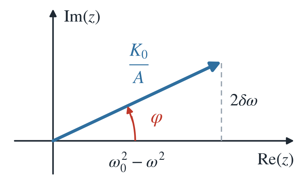
With the Pythagorean theorem (see Figure 2.14) we obtain \[ \left[ \omega_0^2 - \omega^2 \right]^2 + \left[ 2\delta \omega \right]^2 = \left[ \frac{K_0}{A} \right]^2 \tag{2.21}\] and \[ \tan(\varphi) = \frac{2\delta \omega}{\omega_0^2 - \omega^2}. \tag{2.22}\] From Equation 2.21 and Equation 2.22, the amplitude \(A\) and the phase angle \(\varphi\) can be determined. For the amplitude we have \[ A = \frac{K_0}{\sqrt{(\omega_0^2 - \omega^2)^2 + (2\delta \omega)^2}} = \frac{F_0}{m \sqrt{(\omega_0^2 - \omega^2)^2 + (2\delta \omega)^2}}. \tag{2.23}\] For the phase angle \(\varphi\) we distinguish three cases:
- \(\omega < \omega_0\): \(\varphi = \arctan\left(\frac{2\delta \omega}{\omega_0^2 - \omega^2}\right)\), see Figure 2.15 (a).
- \(\omega = \omega_0\): \(\varphi = \frac{\pi}{2}\), see Figure 2.15 (b).
- \(\omega > \omega_0\): \(\varphi = \arctan\left(\frac{2\delta \omega}{\omega_0^2 - \omega^2}\right) + \pi\), see Figure 2.15 (c).
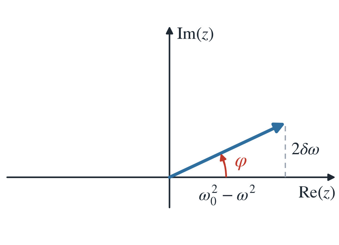
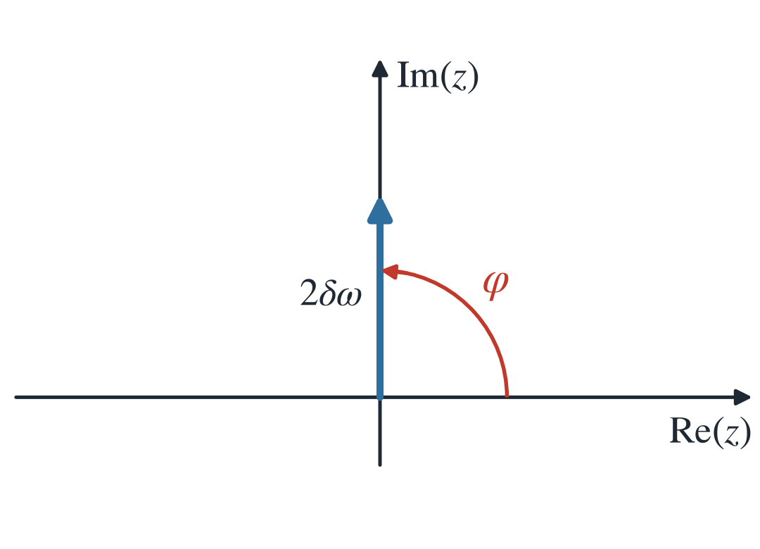
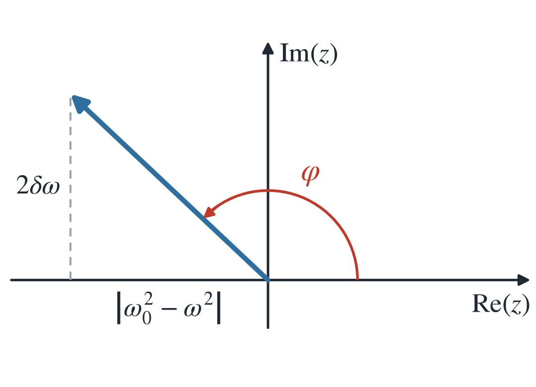
The particular solution of the ODE Equation 2.17 then reads, in complex form, \[ \underline{x}_{\mathrm{p}} = A \mathrm{e}^{\mathrm{j}(\omega t - \varphi)} \] with the amplitude \(A\) from Equation 2.23 and the phase angle \(\varphi\). The sought real solution is its imaginary part: \[ x_{\mathrm{p}} = \operatorname{Im}(\underline{x}_{\mathrm{p}}) = A \sin(\omega t - \varphi). \] Under weak damping (\(\delta < \omega_0\)), the equation of motion Equation 2.17 therefore has the general solution \[ x(t) = x_{\mathrm{h}} + x_{\mathrm{p}} = A_{\mathrm{d}} \mathrm{e}^{-\delta t} \sin(\omega_{\mathrm{d}} t + \varphi_{\mathrm{d}}) + A \sin(\omega t - \varphi). \] The motion of the weakly damped system is thus composed of two oscillations that superpose without disturbing each other.
The homogeneous equation of motion \(\ddot{x} + 2\delta \dot{x} + \omega_0^2 x = 0\) provides the contribution \[ x_{\mathrm{h}}(t) = A_{\mathrm{d}} \mathrm{e}^{-\delta t} \sin(\omega_{\mathrm{d}} t + \varphi_{\mathrm{d}}), \tag{2.24}\] a damped oscillation with the natural angular frequency \(\omega_{\mathrm{d}} = \sqrt{\omega_0^2 - \delta^2}\). Since it is damped, it dies out after a certain time, the transient phase. It is therefore also called the “transient component”, see Figure 2.16.
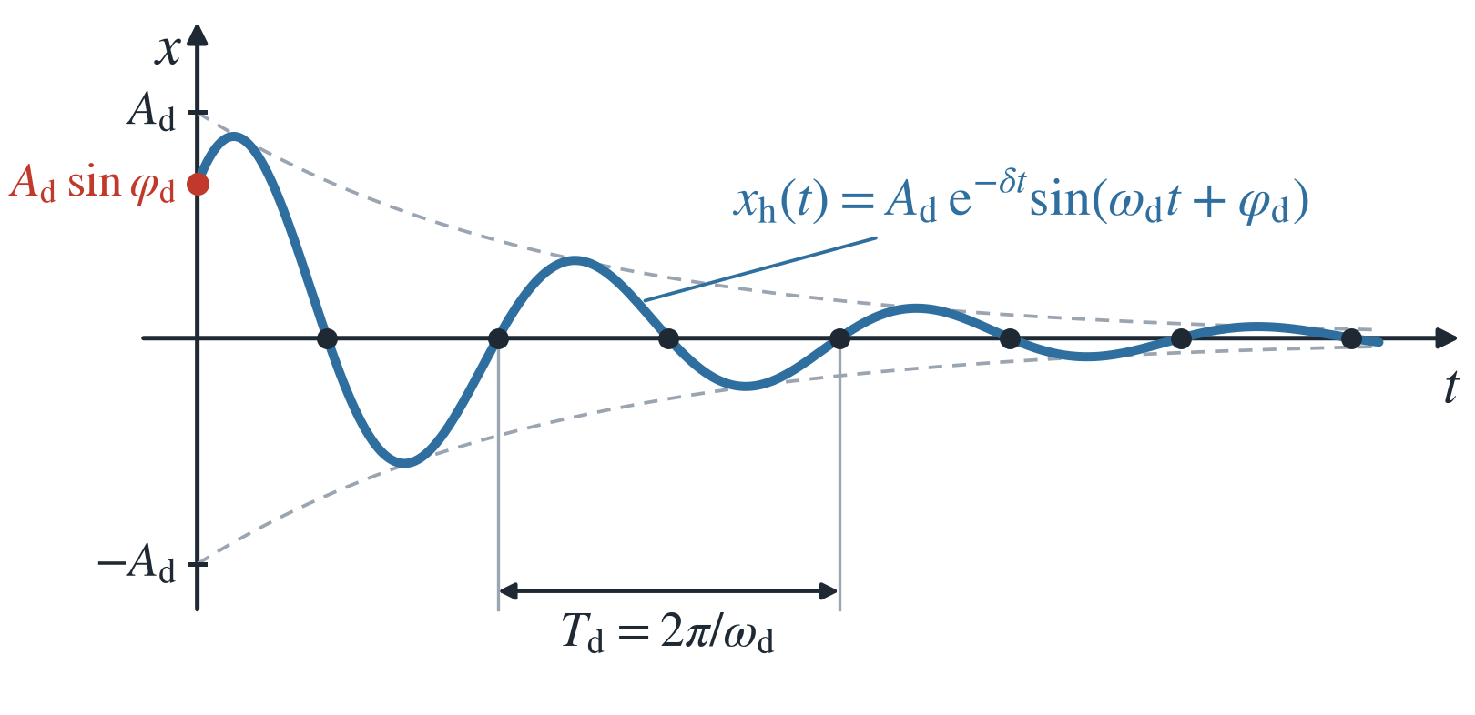
The contribution of the inhomogeneous equation of motion \(\ddot{x} + 2\delta \dot{x} + \omega_0^2 x = K_0 \sin(\omega t)\) to the total oscillation is the particular solution \[ x_{\mathrm{p}}(t) = A \sin(\omega t - \varphi), \tag{2.25}\] an undamped oscillation with the angular frequency \(\omega\) of the exciter. The external force \(F(t)\) thus excites the system to a harmonic oscillation, see Figure 2.17. Such a contribution is called a “forced oscillation”.
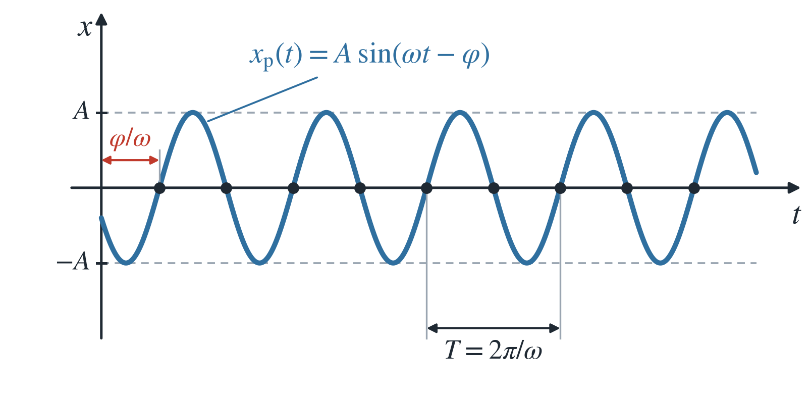
After the transient phase, the transient component of the solution has vanished, so that only the forced oscillation remains, see Figure 2.18.
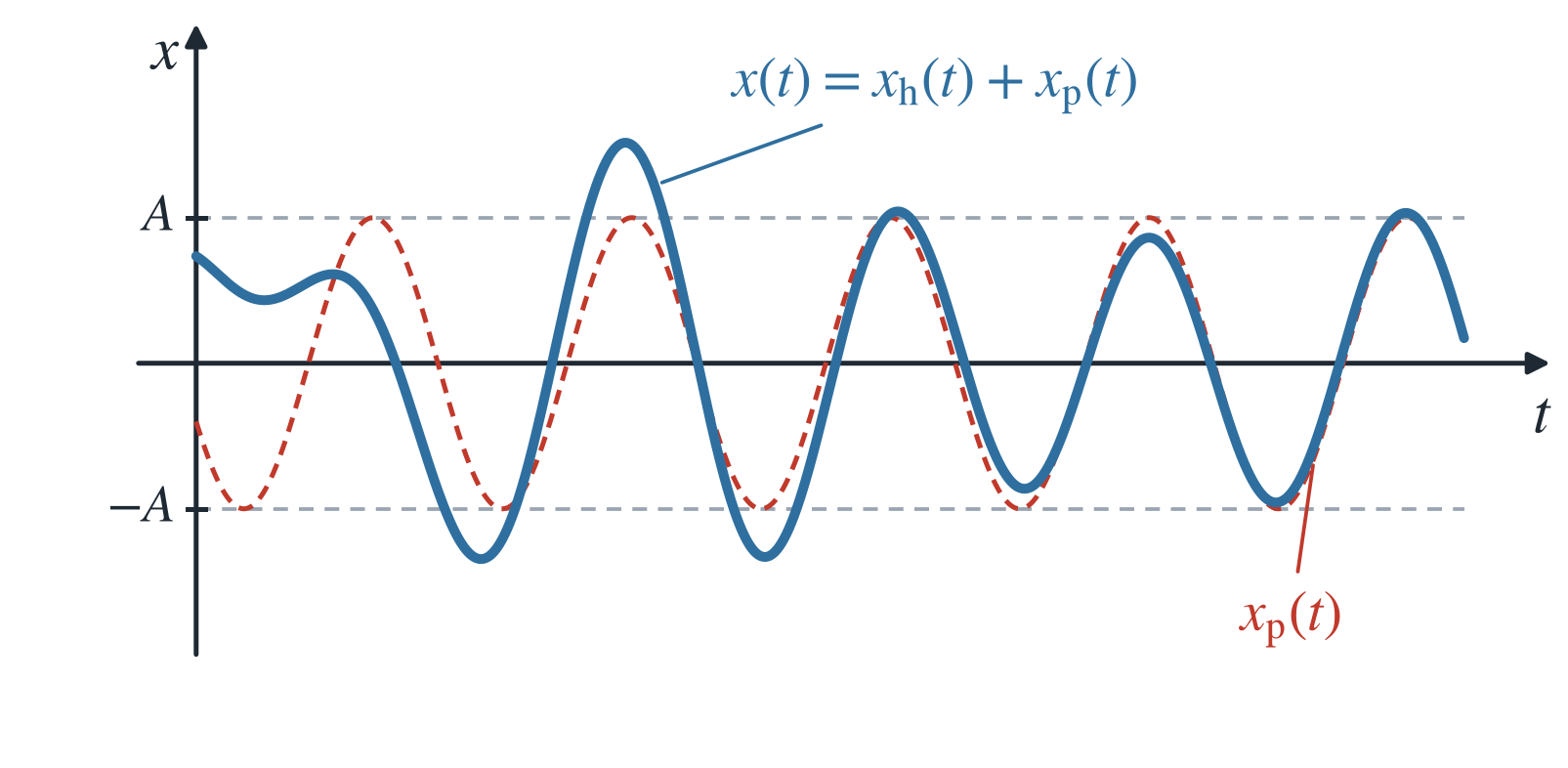
The mechanical system then oscillates without damping at the angular frequency \(\omega\) of the exciter. The amplitude and the phase shift \(\varphi\) between the excitation and the steady-state solution \(x_{\mathrm{p}}(t)\) depend on the excitation angular frequency, \(A = A(\omega)\) and \(\varphi = \varphi(\omega)\).
Example 2.44 (Forced Oscillation) This numerical example is not taken from Papula (2015). It uses characteristic data similar to Example 2.37. A mass-spring oscillator with \(m = 10\) kg, \(b = 40\) kg/s, and \(c = 250\) N/m is excited by the force \(F(t) = 100\,\text{N} \cdot \sin(3\,\text{s}^{-1} \cdot t)\) and starts from the rest position, \(x(0) = 0\) and \(v(0) = 0\). We omit the units in the intermediate calculations. With \[ \delta = \frac{b}{2m} = 2, \qquad \omega_0 = \sqrt{\frac{c}{m}} = 5, \qquad K_0 = \frac{F_0}{m} = 10, \qquad \omega = 3 \] the equation of motion Equation 2.17 reads \[ \ddot{x} + 4\dot{x} + 25x = 10 \sin(3t). \] Since \(\delta < \omega_0\), the system is weakly damped with \(\omega_{\mathrm{d}} = \sqrt{25 - 4} = \sqrt{21}\). By Equation 2.23 and Equation 2.22, the amplitude and the phase angle of the forced oscillation are \[ A = \frac{10}{\sqrt{(25 - 9)^2 + (2 \cdot 2 \cdot 3)^2}} = \frac{10}{\sqrt{256 + 144}} = \frac{10}{20} = 0.5 \] and, since \(\omega < \omega_0\), \[ \varphi = \arctan\left( \frac{12}{16} \right) = \arctan\left( \frac{3}{4} \right) \approx 0.6435, \] i.e., \(\sin\varphi = 3/5\) and \(\cos\varphi = 4/5\). In the form of Theorem 2.10, the general solution is \[ x(t) = \mathrm{e}^{-2t} \left[ C_1 \sin(\sqrt{21}\, t) + C_2 \cos(\sqrt{21}\, t) \right] + 0.5 \sin(3t - \varphi). \] From \(x(0) = C_2 - 0.5 \sin\varphi = C_2 - 0.3 = 0\) it follows that \(C_2 = 0.3\). From \[ \dot{x}(0) = \sqrt{21}\, C_1 - 2 C_2 + 1.5 \cos\varphi = \sqrt{21}\, C_1 - 0.6 + 1.2 = 0 \] it follows that \(C_1 = -0.6/\sqrt{21} \approx -0.1309\). The particular solution is therefore \[ x(t) = \mathrm{e}^{-2t} \left[ -0.1309 \sin(\sqrt{21}\, t) + 0.3 \cos(\sqrt{21}\, t) \right] + 0.5 \sin(3t - 0.6435) \] (in m, \(t \geq 0\)). Since \(\mathrm{e}^{-2t} < 0.01\) for \(t > 2.3\) s, the transient component has practically died out by then. Afterwards, the system oscillates in steady state with the amplitude \(0.5\) m and the excitation angular frequency \(3\,\text{s}^{-1}\), lagging behind the excitation by \(\varphi/\omega \approx 0.21\) s.
2.7.7 Frequency Response
Definition 2.11 (Frequency Response) The dependence of the amplitude \(A\) and the phase shift \(\varphi\) of the forced oscillation on the excitation angular frequency \(\omega\) is called the frequency response. The function \(A(\omega)\) is called the amplitude frequency response, the function \(\varphi(\omega)\) the phase frequency response.
2.7.7.1 Frequency Response of the Amplitude
By Equation 2.23, the amplitude of the forced oscillation is \[ A(\omega) = \frac{F_0}{m \sqrt{(\omega_0^2 - \omega^2)^2 + (2\delta \omega)^2}}. \tag{2.26}\] This function is also called the resonance curve. Its value at \(\omega = 0\) describes the static case.
Definition 2.12 (Static Case) The static case is the limiting case \(\omega \to 0\) of the forced oscillation. The excitation force then changes so slowly that at every instant it acts like a force that is constant in time. A constant force \(F_0\) stretches the spring by the static displacement \[ x_{\mathrm{st}} = \frac{F_0}{c}. \tag{2.27}\]
Remark 2.5 (Remark on the Static Case). Strictly speaking, the excitation force \(F_0 \sin(\omega t)\) vanishes for \(\omega = 0\). What is meant is therefore the limit \(\omega \to 0\): the period \(2\pi/\omega\) of the excitation becomes arbitrarily long, and the force passes through its values between \(-F_0\) and \(F_0\) arbitrarily slowly. In the static case, the resonance curve has the value \[ A(0) = \frac{F_0}{m \omega_0^2} = \frac{F_0}{c} = x_{\mathrm{st}}. \]
A plausible explanation follows from comparing the three forces in the equation of motion \(m\ddot{x} + b\dot{x} + cx = F(t)\). For the steady-state solution \(x = A \sin(\omega t - \varphi)\), the inertial force \(m\ddot{x}\), the damping force \(b\dot{x}\), and the spring force \(cx\) have the amplitudes \[ m A \omega^2, \qquad b A \omega \qquad \text{and} \qquad c A. \] For \(\omega \to 0\), the first two become arbitrarily small compared with the spring force, and the equation of motion turns into Hooke’s law \(c\,x = F(t)\) (Theorem 2.7). The mass is moved so slowly that neither its inertia nor the damper plays a role; the spring alone balances the external force. This is why \(A(0)\) depends neither on the mass \(m\) nor on the damping \(\delta\), and why all resonance curves in Figure 2.19 start at the same point. For the same reason, the displacement follows the force without delay; the phase shift is \(\varphi(0) = 0\) (Section 2.7.7.2).
In the static case, the mass-spring oscillator looks as in Figure 2.2, with the force \(F(t) = F_0\) pulling downward constantly. The mass rests in a new equilibrium position that lies \(x_{\mathrm{st}} = F_0/c\) below the original rest position \(x = 0\). The spring is stretched by this amount in addition, and the piston of the damper stands still. The system acts like a spring balance that indicates the force \(F_0\) by the extension of the spring.
For the behavior, we distinguish two situations:
- Constant force. If the force \(F_0\) is switched on at time \(t = 0\) while the mass rests at the rest position \(x = 0\), then by Table 2.2 (polynomial of degree \(0\)), \(x_{\mathrm{p}} = F_0/c\) is a particular solution of \(\ddot{x} + 2\delta \dot{x} + \omega_0^2 x = F_0/m\). The general solution is \(x(t) = x_{\mathrm{h}}(t) + F_0/c\). The component \(x_{\mathrm{h}}\) of the homogeneous ODE describes a transient motion that, depending on the damping (Table 2.3), dies out as a damped oscillation about \(x_{\mathrm{st}}\) or as a creeping motion. Afterwards, the mass stays at the position \(x_{\mathrm{st}}\).
- Very slowly varying force. If the force \(F(t) = F_0 \sin(\omega t)\) changes with a very small excitation angular frequency \(\omega \ll \omega_0\), the mass passes through the equilibrium positions \(x(t) \approx F(t)/c\) one after another. It moves in step with the force between \(-x_{\mathrm{st}}\) and \(x_{\mathrm{st}}\) without oscillating noticeably at its natural frequency. Such a motion is called quasi-static.
The static displacement serves as the reference quantity for the resonance curve: the ratio \(A(\omega)/x_{\mathrm{st}}\) states by which factor the periodic excitation increases the displacement compared with the static case. In Example 2.44, \(x_{\mathrm{st}} = 100\,\mathrm{N}/(250\,\mathrm{N/m}) = 0.4\) m. At \(\omega = 3\,\text{s}^{-1}\), the amplitude is \(0.5\) m, so the displacement is larger than in the static case by the factor \(1.25\).
The maximum of the resonance curve lies where the radicand in the denominator of Equation 2.26, \[ \Psi(\omega) = (\omega_0^2 - \omega^2)^2 + (2\delta \omega)^2, \] becomes minimal. From the condition \[ \Psi'(\omega) = 4 \omega (\omega^2 - \omega_0^2 + 2\delta^2) = 0 \] we obtain, for \(\omega > 0\), the minimizer \[ \omega_{\mathrm{r}} = \sqrt{\omega_0^2 - 2\delta^2}, \] which is real only for \(\omega_0^2 > 2\delta^2\). The second derivative \[ \Psi''(\omega) = 4(3\omega^2 - \omega_0^2 + 2\delta^2) \] is positive at this point: \[ \Psi''(\omega_{\mathrm{r}}) = 4(3\omega_{\mathrm{r}}^2 - \omega_0^2 + 2\delta^2) = 8 (\omega_0^2 - 2\delta^2) > 0. \]
At \(\omega_{\mathrm{r}}\), the resonance curve \(A(\omega)\) therefore has a maximum. The angular frequency \(\omega_{\mathrm{r}}\) is called the resonance frequency, the amplitude \(A_{\mathrm{r}} = A(\omega_{\mathrm{r}})\) the resonance amplitude. In the presence of damping, the resonance frequency is always smaller than \(\omega_{\mathrm{d}}\) and hence smaller than the natural angular frequency \(\omega_0\): \[ \omega_{\mathrm{r}} = \sqrt{\omega_0^2 - 2\delta^2} < \omega_{\mathrm{d}} = \sqrt{\omega_0^2 - \delta^2} < \omega_0. \] If the excitation angular frequency equals the resonance frequency, \(\omega = \omega_{\mathrm{r}}\), the system oscillates with the largest possible amplitude. This resonance case yields the resonance amplitude \[ A_{\mathrm{r}} = A_{\max} = A(\omega_{\mathrm{r}}) = \frac{F_0}{2m \delta \sqrt{\omega_0^2 - \delta^2}} = \frac{F_0}{2m \delta \omega_{\mathrm{d}}}. \]
With increasing excitation angular frequency \(\omega\), the amplitude \(A(\omega)\) decreases and tends to zero as \(\omega \to \infty\). The system is then no longer able to follow the rapid changes of the excitation force. Figure 2.19 shows the resonance curve for three dampings.
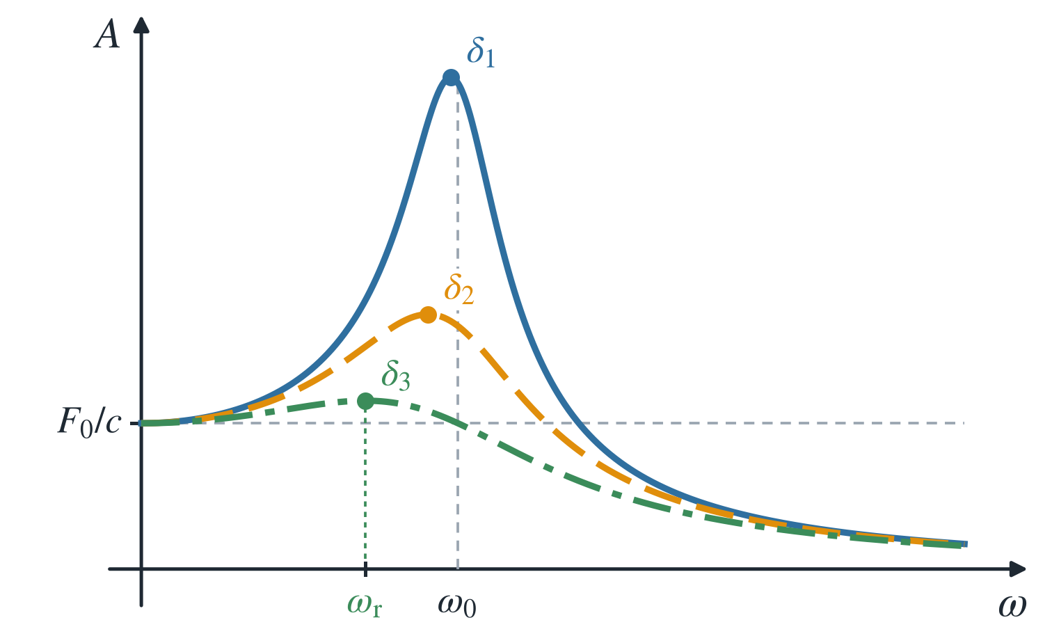
In summary, we obtain the important result for the resonance case:
Theorem 2.13 (Resonance Case) The resonance case occurs when the excitation angular frequency \(\omega\) equals the resonance frequency \[ \omega_{\mathrm{r}} = \sqrt{\omega_0^2 - 2\delta^2} \] The system then oscillates with the largest possible amplitude, the resonance amplitude \(A_{\mathrm{r}}\).
2.7.7.2 Frequency Response of the Phase Shift
By Equation 2.25, the forced oscillation always lags behind the excitation oscillation by the phase angle \(\varphi\), where \(\varphi\) lies between \(0\) and \(\pi\). Figure 2.20 shows the frequency response of the phase shift \(\varphi(\omega)\).
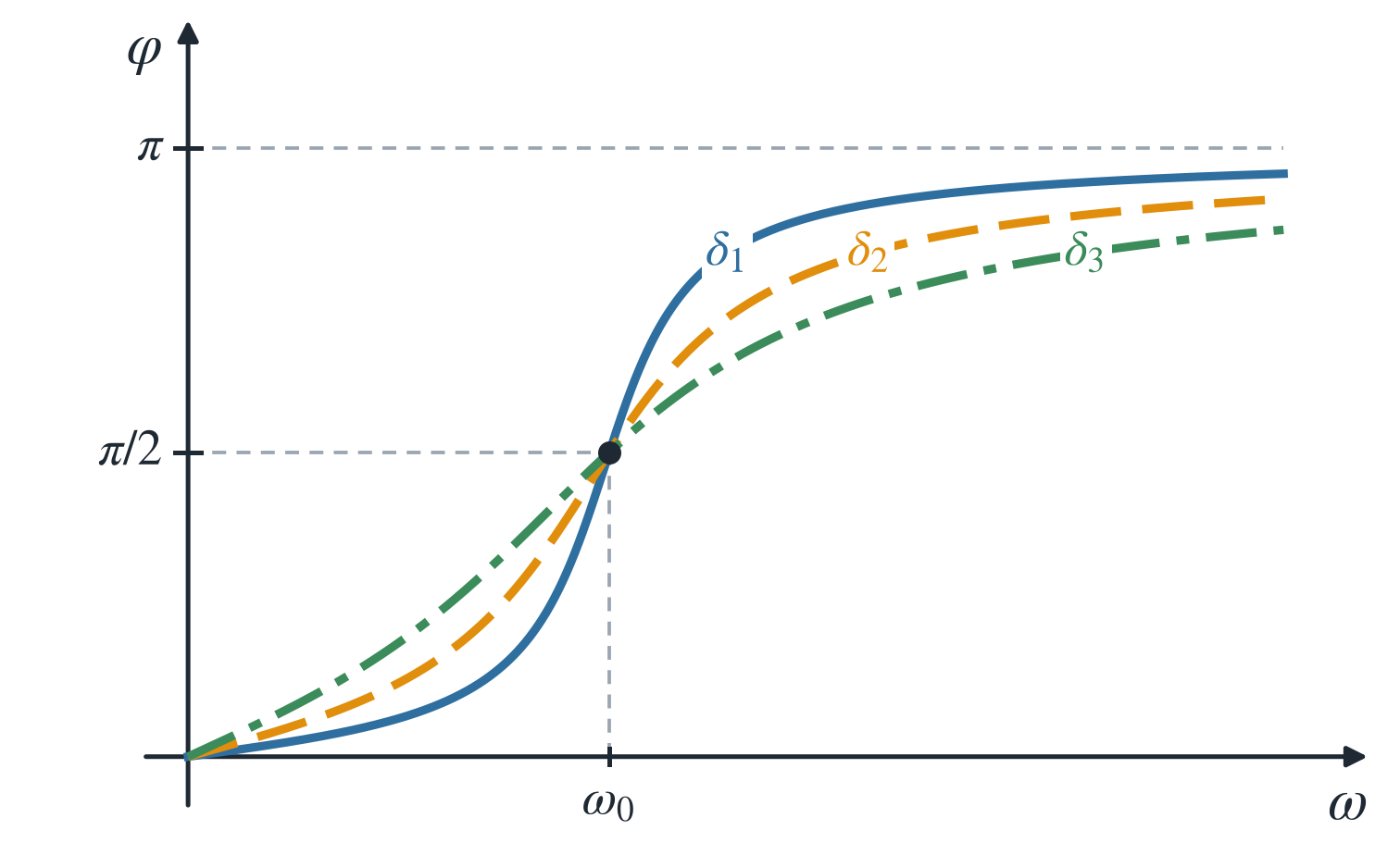
In the static case (\(\omega = 0\)) the phase shift is \(\varphi(0) = 0\), for \(\omega = \omega_0\) it is \(\varphi(\omega_0) = \pi/2\), and for \(\omega \to \infty\) it is \(\varphi(\infty) = \pi\). For high angular frequencies, the oscillation therefore lags behind the excitation oscillation by \(\pi\): exciter and system oscillate in antiphase.
Example 2.45 (Frequency Response in the Absence of Damping and under Strong Damping) We investigate the frequency response of the amplitude \(A(\omega)\) and of the phase shift \(\varphi(\omega)\) in the absence of damping (\(\delta = 0\)) and under strong damping (\(\delta > \omega_0\)). The basis is the resonance curve Equation 2.26 and the phase relation \[ \tan(\varphi) = \frac{2\delta \omega}{\omega_0^2 - \omega^2}, \qquad 0 \le \varphi \le \pi. \]
No damping (\(\delta = 0\)). The resonance curve simplifies to \[ A(\omega) = \frac{F_0}{m\,\lvert \omega_0^2 - \omega^2 \rvert} \qquad (\omega \neq \omega_0). \] It starts in the static case at \(A(0) = F_0/(m\omega_0^2) = x_{\mathrm{st}}\), increases monotonically for \(0 < \omega < \omega_0\), and tends to infinity as \(\omega \to \omega_0\). For \(\omega > \omega_0\), it decreases monotonically and tends to zero as \(\omega \to \infty\). The resonance frequency \(\omega_{\mathrm{r}} = \sqrt{\omega_0^2 - 2\delta^2}\) coincides with the natural angular frequency \(\omega_0\). A finite resonance amplitude does not exist. At \(\omega = \omega_0\), the excitation is a solution of the homogeneous ODE. By Table 2.2, the ansatz with the factor \(t\) must then be chosen, which yields the particular solution \[ x_{\mathrm{p}}(t) = -\frac{F_0}{2m\omega_0}\, t \cos(\omega_0 t). \] Its amplitude grows linearly with time beyond all bounds. This case is called a resonance catastrophe. A real system is destroyed by it unless damping prevents it.
The numerator \(2\delta\omega\) of the phase relation vanishes, so \(\tan(\varphi) = 0\) for all \(\omega \neq \omega_0\). For \(\omega < \omega_0\), the denominator is positive and \(\varphi = 0\): the system oscillates in phase with the excitation. For \(\omega > \omega_0\), the denominator is negative and \(\varphi = \pi\): the system oscillates in antiphase. At \(\omega = \omega_0\), the phase response jumps from \(0\) to \(\pi\). It is the limit of the curves in Figure 2.20 as \(\delta \to 0\).
Strong damping (\(\delta > \omega_0\)). We write the radicand in the denominator of Equation 2.26 as a polynomial in \(\omega^2\), \[ \Psi(\omega) = \omega^4 + 2\left(2\delta^2 - \omega_0^2\right)\omega^2 + \omega_0^4. \] Since \(\delta > \omega_0\), we have \(2\delta^2 - \omega_0^2 > \delta^2 > 0\). All coefficients are positive, so \(\Psi\) increases strictly monotonically for \(\omega > 0\) and the amplitude \(A(\omega)\) decreases strictly monotonically. The resonance curve attains its maximum in the static case, \(A(0) = x_{\mathrm{st}}\), and there is no resonance: \(\omega_{\mathrm{r}} = \sqrt{\omega_0^2 - 2\delta^2}\) is not real. This already holds for \(\delta \ge \omega_0/\sqrt{2}\). At the natural angular frequency, the amplitude is \[ A(\omega_0) = \frac{F_0}{2m\delta\omega_0} = \frac{\omega_0}{2\delta}\, x_{\mathrm{st}} < \frac{x_{\mathrm{st}}}{2}, \] and it tends to zero as \(\omega \to \infty\).
As in the case of weak damping, the phase response runs from \(\varphi(0) = 0\) via \(\varphi(\omega_0) = \pi/2\) to \(\varphi(\infty) = \pi\), but it rises noticeably already at small angular frequencies. At \(\omega = \omega_0/2\), \[ \tan(\varphi) = \frac{4\delta}{3\omega_0}. \] For \(\delta > \omega_0\), it follows that \(\varphi > \arctan(4/3) \approx 53^\circ\), whereas the weak damping \(\delta = 0.1\,\omega_0\) reaches only \(\varphi \approx 7.6^\circ\). Under strong damping, the transition from \(0\) to \(\pi\) is therefore spread over a wide frequency range. In Figure 2.20, this tendency is already visible in the curve with the largest damping \(\delta_3\).
2.8 Simple Pendulum
Definition 2.13 (Simple Pendulum) A simple pendulum is a physical model consisting of a mass \(m\) at the end of a massless, inextensible thread of length \(l\). Its position is described by the angle of deflection \(\varphi(t)\) from the vertical rest position.
2.8.1 Equation of Motion
If the pendulum is displaced and released, it oscillates under the influence of gravity. The motion is described by an ODE based on Newton’s second law and on the fact that the restoring force is proportional to the sine of the angle of deflection (Figure 2.21). With the weight force \(F_{\mathrm{G}} = mg\) and the gravitational acceleration \(g\), the restoring force \(F_{\mathrm{R}}\) is \[ F_{\mathrm{R}} = F_{\mathrm{G}} \sin(\varphi) = m g \sin(\varphi). \] With the arc length \(s(t)\), the equation of motion reads \[ F = m \ddot{s} = - m g \sin \varphi(t). \] Because \[ \varphi(t) = \frac{s(t)}{l} \] it can be formulated in terms of \(s(t)\) alone, \[ F = m \ddot{s} = - m g \sin\left(\frac{s}{l}\right), \] or in terms of the angle of deflection \(\varphi(t)\) alone: \[ F = m l \ddot{\varphi} = - m g \sin(\varphi). \tag{2.28}\]
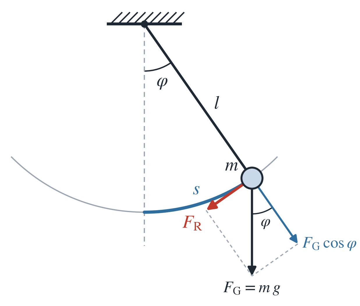
The simple pendulum sketched in Figure 2.21 oscillates almost harmonically for small displacements. Rearranging Equation 2.28 yields the ODE \[ \ddot{\varphi} + \frac{g}{l}\sin(\varphi) = 0. \tag{2.29}\] In simplified form we obtain the representation in Figure 2.22.
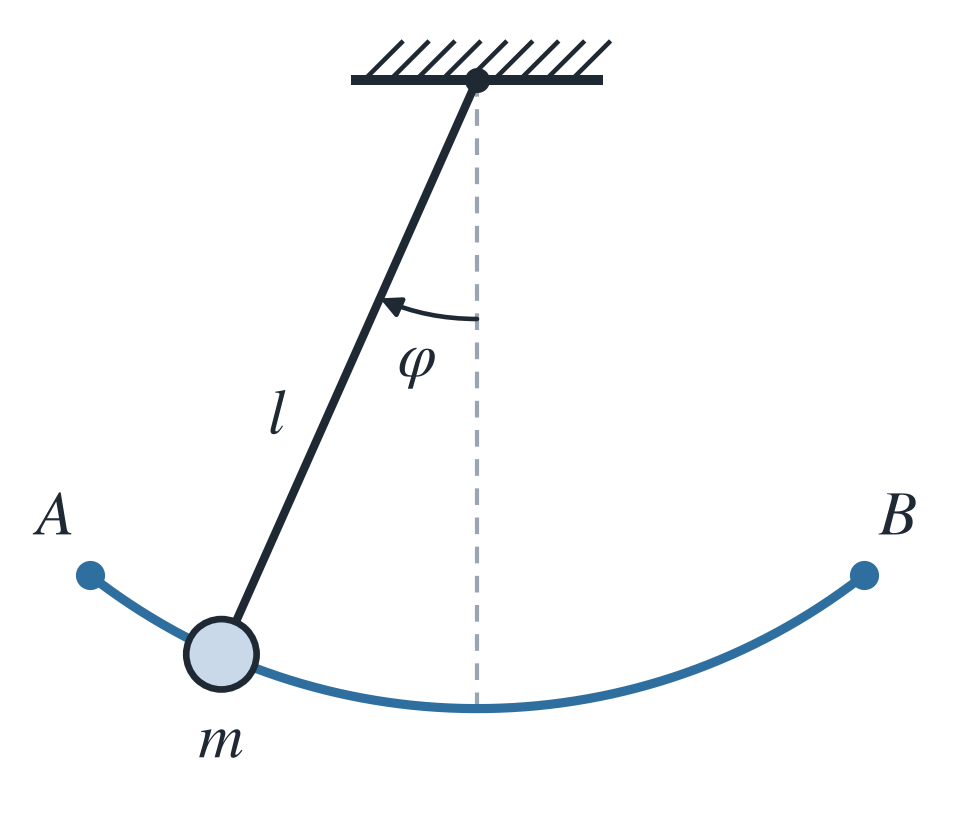
For small displacements \(\varphi\), \(\sin(\varphi) \approx \varphi\), so that Equation 2.29 approximately takes the form \[ \ddot{\varphi} + \frac{g}{l} \varphi = 0 \tag{2.30}\] With \(\omega_0^2 = g/l\), the ODE reads \[ \ddot{\varphi} + \omega_0^2 \varphi = 0. \tag{2.31}\]
2.8.2 The General Solution of the Equation of Motion
The characteristic equation \[ \lambda^2 + \omega_0^2 = 0 \] has the solutions \[ \lambda_{1,2} = \pm \mathrm{j} \omega_0. \] The general solution of Equation 2.31 is \[ \varphi(t) = C_1 \sin(\omega_0 t) + C_2 \cos(\omega_0 t) \] with the time derivative \[ \dot{\varphi}(t) = \omega_0 \left[ C_1 \cos(\omega_0 t) - C_2 \sin(\omega_0 t) \right]. \] The simple pendulum oscillates with the angular frequency \[ \omega_0 = \sqrt{\frac{g}{l}}, \] the frequency \[ \nu_0 = \frac{\omega_0}{2\pi} = \frac{1}{2\pi} \sqrt{\frac{g}{l}} \] and the period \[ T_0 = 2\pi \sqrt{\frac{l}{g}}. \]
Example 2.46 (Simple Pendulum: Motion Starting from Rest) For the initial conditions \(\varphi(0) = \varphi_0\) and \(\dot{\varphi}(0) = 0\), the pendulum starts from rest. Since \(\varphi(0) = C_2 = \varphi_0\) and \(\dot{\varphi}(0) = \omega_0 C_1 = 0\), i.e., \(C_1 = 0\), the particular solution is \[ \varphi(t) = \varphi_0 \cos(\omega_0 t), \quad t \geq 0. \]
A pendulum that oscillates only at small angles is a rather uninteresting pendulum. Unfortunately, for the pendulum equation Equation 2.29 at large angles there is no explicit solution that is algebraically as simple. Since this system is much simpler than most engineering systems and still has no simple analytical solution, the need for numerical solution methods for ODEs becomes clear.
2.9 Reduction of Order
We consider a vector \(S(t)\) that represents the state of a system as a function of time \(t\). In general, the state comprises all dependent variables that are relevant to the behavior of the system. For an initial value problem of the ODE of order \(n\) \[ y^{(n)}(t) = f\left(t, y(t), y'(t), y''(t), \dots, y^{(n-1)}(t)\right) \] we define the state as \[ S(t) = \left[\begin{array}{c} y(t) \\ y'(t) \\ y''(t) \\ \vdots \\ y^{(n-1)}(t) \end{array}\right]. \] The derivative of the state is then \[ \frac{\mathrm{d}S(t)}{\mathrm{d}t} = \left[\begin{array}{c} y'(t) \\ y''(t) \\ \vdots \\ y^{(n-1)}(t) \\ y^{(n)}(t) \end{array}\right] = \left[\begin{array}{c} y'(t) \\ y''(t) \\ \vdots \\ y^{(n-1)}(t) \\ f\left(t, y(t), y'(t), \dots, y^{(n-1)}(t)\right) \end{array}\right] = \left[\begin{array}{c} S_2(t) \\ S_3(t) \\ \vdots \\ S_n(t) \\ f\left(t, S_1(t), S_2(t), \dots, S_n(t)\right) \end{array}\right], \] where \(S_i(t)\) is the \(i\)-th component of \(S(t)\). In this description, \(\frac{\mathrm{d}S(t)}{\mathrm{d}t}\) can be expressed in terms of \(S(t)\) alone, without \(y(t)\) and its derivatives. If \(f\) now denotes the vector-valued right-hand side, then \[ \frac{\mathrm{d}S(t)}{\mathrm{d}t} = f(t, S(t)). \] This equation is a first-order ODE in \(S\): we have converted an ODE of order \(n\) into \(n\) coupled first-order ODEs.
Example 2.47 (Coupled Differential Equations) A very simple model to describe the change in the populations of rabbits, \(r(t)\), and wolves, \(w(t)\), could be
\[ \frac{\mathrm{d}r(t)}{\mathrm{d}t} = 4r(t) - 2w(t) \tag{2.32}\]
and
\[ \frac{\mathrm{d}w(t)}{\mathrm{d}t} = r(t) + w(t). \tag{2.33}\]
Equation 2.32 states that at each time step the rabbit population quadruples, but each wolf eats two of the rabbits. Equation 2.33 states that at each time step the population of wolves increases by the number of rabbits and wolves in the system. We write this system of differential equations as an equivalent differential equation in \(S(t)\).
To do so, we combine the two populations in the state vector \[ S(t) =\left[\begin{array}{c} r(t) \\ w(t) \end{array}\right]. \] We form its derivative componentwise and substitute Equation 2.32 and Equation 2.33: \[ \frac{\mathrm{d}S(t)}{\mathrm{d}t} = \left[\begin{array}{c} \frac{\mathrm{d}r(t)}{\mathrm{d}t} \\ \frac{\mathrm{d}w(t)}{\mathrm{d}t} \end{array}\right] = \left[\begin{array}{c} 4r(t) - 2w(t) \\ r(t) + w(t) \end{array}\right]. \] The right-hand side is linear in \(r(t)\) and \(w(t)\) in both components. We thus write it as the product of a coefficient matrix and \(S(t)\): the first row contains the coefficients \(4\) and \(-2\) of Equation 2.32, the second row the coefficients \(1\) and \(1\) of Equation 2.33. The first-order differential equation \[ \frac{\mathrm{d}S(t)}{\mathrm{d}t} = \left[\begin{array}{cc} 4 & -2 \\ 1 & 1 \end{array}\right]S(t) \tag{2.34}\] is therefore equivalent to the pair of differential equations. Multiplying out the right-hand side recovers Equation 2.32 and Equation 2.33.
Equation 2.34 is a coupled ODE.
Definition 2.14 (Coupled ODE) A system of ODEs in which one or more unknowns appear in more than one equation is called coupled. The equations then depend on each other.
Many numerical methods for initial value problems are designed for first-order ODEs. To use them for higher-order ODEs, their order is reduced to one. To this end, new variables are introduced for the derivatives of the original function up to the \((n-1)\)-th order, which converts an ODE of order \(n\) into a system of \(n\) first-order ODEs.
Theorem 2.14 (Reduction of Order) Consider an ODE of order \(n\) in the form \[ y^{(n)} = f\left(t, y, y', y'', \dots, y^{(n-1)}\right). \] With the \(n\) new variables \[\begin{align*} y_1 &= y,\\ y_2 &= y',\\ y_3 &= y'',\\ &\;\;\vdots\\ y_n &= y^{(n-1)}, \end{align*}\] each of which corresponds to a derivative of the original function \(y\), it is equivalent to the system of \(n\) first-order ODEs consisting of the \(n-1\) equations \[\begin{align*} y_1' &= y_2,\\ y_2' &= y_3,\\ &\;\;\vdots\\ y_{n-1}' &= y_n \end{align*}\] and the equation \[ y_n' = f(t, y_1, y_2, y_3, \dots, y_n) \tag{2.35}\]
Proof. The first \(n-1\) equations follow from the definition of the \(y_i\). The last equation is the original ODE expressed in terms of the \(y_i\).
The system contains only the \(y_i\) and can be solved with the usual numerical methods for systems of first-order ODEs, e.g., with the Runge-Kutta methods.
In vector form, the variables and their derivatives with respect to time \(t\) are collected into \[ S = \begin{pmatrix} y_1 \\ y_2 \\ \vdots \\ y_n \end{pmatrix} \quad \text{and} \quad S' = \begin{pmatrix} y_1' \\ y_2' \\ \vdots \\ y_n' \end{pmatrix} \] A linear system can then be written in matrix form as \[ S' = AS + g(t), \] where \(A\) is an \(n \times n\) matrix of the coefficients and the vector function \(g(t)\) describes external influences or inhomogeneous terms. If the right-hand side in Equation 2.35 is linear, \(f = a_1 y_1 + a_2 y_2 + \dots + a_n y_n\), and no external influences act, then \(g(t) = 0\) is the zero vector. The matrix \(A\) then has the form \[ A = \begin{pmatrix} 0 & 1 & 0 & \cdots & 0 \\ 0 & 0 & 1 & \cdots & 0 \\ \vdots & \vdots & \vdots & \ddots & \vdots \\ 0 & 0 & 0 & \cdots & 1 \\ a_1 & a_2 & a_3 & \cdots & a_n \end{pmatrix}. \]
Example 2.48 (Reduction of Order) Consider the second-order ODE \[ y'' = -\omega_0^2 y. \] With the new variables \[\begin{align*} y_1 &= y, \\ y_2 &= y' \end{align*}\] we obtain, since the derivative of \(y_1\) equals \(y_2\), the system \[\begin{align*} y_1' &= y_2,\\ y_2' &= -\omega_0^2 y_1. \end{align*}\] It consists of two first-order ODEs that are equivalent to the original second-order ODE and can be solved with numerical methods. With \[ S = \begin{pmatrix} y_1 \\ y_2 \end{pmatrix}, \quad S' = \begin{pmatrix} y_1' \\ y_2' \end{pmatrix} = \begin{pmatrix} y_2 \\ -\omega_0^2 y_1 \end{pmatrix}, \quad A = \begin{pmatrix} 0 & 1 \\ -\omega_0^2 & 0 \end{pmatrix} \quad \text{and} \quad g(t) = 0 \] it reads in matrix form \[ \begin{pmatrix} y_1' \\ y_2' \end{pmatrix} = \begin{pmatrix} 0 & 1 \\ -\omega_0^2 & 0 \end{pmatrix} \begin{pmatrix} y_1 \\ y_2 \end{pmatrix}. \]
Example 2.49 (Reduction of Order of the Differential Equation of the Simple Pendulum) The second-order ODE of the simple pendulum Equation 2.30, \[ \ddot{\varphi} + \frac{g}{l} \varphi = 0, \] reads, after rearranging, \[ \ddot{\varphi} = -\frac{g}{l} \varphi. \] We set \[ y_1 = \varphi, \quad y_2 = \dot{\varphi}. \tag{2.36}\] By Equation 2.36, differentiating \(y_1\) yields \(y_1' = y_2\). We thus obtain the first-order system \[\begin{align*} y_1' &= y_2,\\ y_2' &= -\frac{g}{l} y_1 \end{align*}\] or, in matrix form with \(S = (y_1, y_2)^T\), \[ \frac{\mathrm{d}S(t)}{\mathrm{d}t} = \begin{pmatrix} 0 & 1\\ -\frac{g}{l} & 0 \end{pmatrix} S(t). \tag{2.37}\]
Although the reduction of order leads to a system with several variables, all derivatives are still taken with respect to the same independent variable, e.g., \(t\). Hence we again obtain a system of ordinary differential equations.