---
jupyter: python3
---
# Systems of Second-Order Linear Differential Equations in Python
@tbl-symbole-07 summarizes the symbols of this chapter together with their type and the place where they are defined.
| Symbol | Meaning | Type | Defined in |
|:--|:--|:--|:--|
| $c$ | Spring constant | Constant | @thm-hookesches-gesetz |
| $c_i$ | Spring constant of spring $i$ ($c_{12}$: coupling spring) | Constant | @exm-eigenwerte-eigenvektoren, @sec-gekoppelte-federn-python |
| $\mathrm{d}$ | Differential ($\mathrm{d}x$, $\frac{\mathrm{d}y}{\mathrm{d}x}$) | Operator | @sec-dgl-systeme-python-einfuehrung |
| $f_1, f_2$ | Right-hand sides of a system of two second-order ODEs | Function | @sec-dgl-systeme-python-einfuehrung |
| $m$ | Mass | Constant | @thm-erstes-newtonsches-gesetz |
| $m_i$ | Mass $i$ | Constant | @sec-gekoppelte-federn-python |
| $t$ | Time | Scalar | @eq-frei-ungedaempft |
| $v$ | Velocity, $v = \dot{x}$; $v_0$ initial velocity | Scalar | @fig-feder-masse-schwinger |
| $x_1, x_2$ | Displacement from the rest position; $x_i$ displacement of mass $i$; $x_0$ initial displacement | Function | @thm-hookesches-gesetz |
| $y_1, \dots, y_4$ | Components of the state vector $S$ in the reduction of order ($y_1 = y$, $y_2 = y'$, …) or of the solution vector $y$ of a system | Function | @thm-reduktion-ordnung |
| local | Unknown functions $x(t)$, $y(t)$ and derivative $w = \mathrm{d}y/\mathrm{d}t$ in the introductory example | local | @sec-dgl-systeme-python-einfuehrung |
| $\dot{x}, \ddot{x}$ | First and second derivative with respect to time $t$ | Operator | @eq-frei-ungedaempft |
: Symbols in Chapter 07 {#tbl-symbole-07}
## Introduction {#sec-dgl-systeme-python-einfuehrung}
A system of second-order linear ODEs can be solved in Python with the function `scipy.integrate.solve_ivp` from the `scipy` library, which was developed specifically for initial value problems of ODE systems.
To this end, a second-order system first has to be converted into a first-order system, because `solve_ivp` and similar functions operate on first-order ODEs.
As an example, consider a system of two second-order ODEs for the unknown functions $x(t)$ and $y(t)$:
\begin{align*}
\frac{\mathrm{d}^2x}{\mathrm{d}t^2} &= f_1\left(x, y, \frac{\mathrm{d}x}{\mathrm{d}t}, \frac{\mathrm{d}y}{\mathrm{d}t}, t\right), \\
\frac{\mathrm{d}^2y}{\mathrm{d}t^2} &= f_2 \left(x, y, \frac{\mathrm{d}x}{\mathrm{d}t}, \frac{\mathrm{d}y}{\mathrm{d}t}, t \right).
\end{align*}
New variables for the first derivatives, $v = \frac{\mathrm{d}x}{\mathrm{d}t}$ and $w = \frac{\mathrm{d}y}{\mathrm{d}t}$, turn it into a system of four first-order ODEs:
\begin{align*}
\frac{\mathrm{d}x}{\mathrm{d}t} &= v, \\
\frac{\mathrm{d}v}{\mathrm{d}t} &= f_1(x, y, v, w, t), \\
\frac{\mathrm{d}y}{\mathrm{d}t} &= w, \\
\frac{\mathrm{d}w}{\mathrm{d}t} &= f_2(x, y, v, w, t).
\end{align*}
::: {#exm-dgl-system-2-ordnung-python}
#### Two Harmonic Oscillators in Python
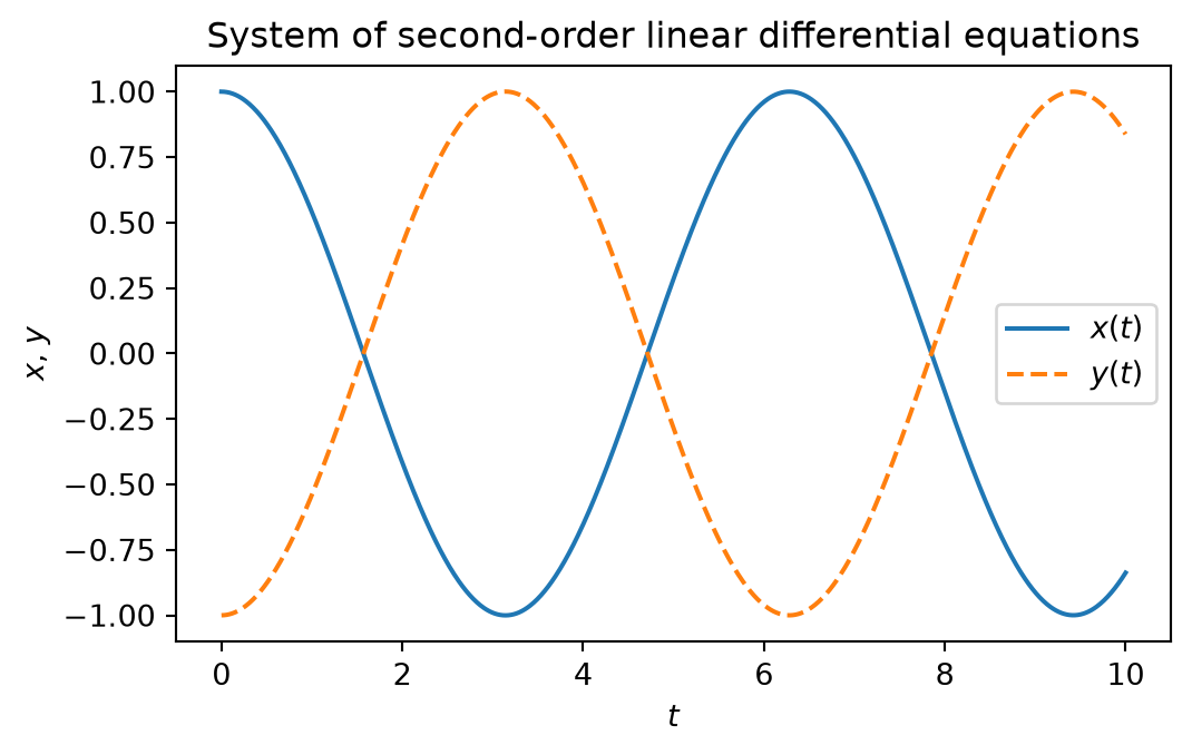
For $f_1 = -x$ and $f_2 = -y$ (two uncoupled harmonic oscillators), the system can be solved in Python as follows:
```{python}
import numpy as np
from scipy.integrate import solve_ivp
import matplotlib.pyplot as plt

# Define the differential equations
def system(t, z):
    x, v, y, w = z
    dxdt = v
    dvdt = -x  # Example for f1: -x
    dydt = w
    dwdt = -y  # Example for f2: -y, a simple harmonic oscillator system
    return [dxdt, dvdt, dydt, dwdt]

# Initial conditions: x(0) = 1, dx/dt(0) = 0, y(0) = -1, dy/dt(0) = 0
z0 = [1.0, 0.0, -1.0, 0.0]

# Time span over which the solution is computed
t_span = (0, 10)
t_eval = np.linspace(*t_span, 1000)

# Solve the ODE system
sol = solve_ivp(system, t_span, z0, t_eval=t_eval)

# Plot the results
plt.plot(sol.t, sol.y[0], label=r'$x(t)$')
plt.plot(sol.t, sol.y[2], label=r'$y(t)$', linestyle='--')
plt.legend()
plt.xlabel(r'$t$')
plt.ylabel(r'$x$, $y$')
plt.title('System of second-order linear differential equations')
plt.show()
```
At each point in time, the state vector `z` contains the quantities $x$, $v$, $y$, and $w$ (in the code `x`, `v`, `y`, `w`). The function `system()` defines the ODE system. `solve_ivp` solves it over the time span `t_span` with the initial conditions `z0`.
The figure shows the curves of $x(t)$ and $y(t)$.
:::
This template can be adapted to a specific system of second-order linear ODEs by changing the expressions for `dvdt` and `dwdt`, i.e., $f_1$ and $f_2$, in the function `system()`.
## Coupled Springs {#sec-gekoppelte-federn-python}
We now solve the equations of motion of the two coupled spring-mass systems from @exm-eigenwerte-eigenvektoren numerically. They have identical masses $m$, identical spring constants $c$, and a coupling spring with spring constant $c_{12}$. By @eq-gekoppelt-1 and @eq-gekoppelt-2, their equations of motion form a system of two coupled second-order ODEs:
\begin{align*}
m \ddot{x}_1 &= -c x_1 - c_{12}(x_1 - x_2),\\
m \ddot{x}_2 &= -c x_2 - c_{12}(x_2 - x_1).
\end{align*}
We generalize it to different masses $m_1$ and $m_2$ and different spring constants $c_1$ and $c_2$ of the two outer springs:
\begin{align*}
m_1 \ddot{x}_1 &= -c_1 x_1 - c_{12}(x_1 - x_2),\\
m_2 \ddot{x}_2 &= -c_2 x_2 - c_{12}(x_2 - x_1).
\end{align*}
To convert it into a first-order system, we introduce, as in @thm-reduktion-ordnung, the state variables $y_1 = x_1$, $y_2 = x_2$, $y_3 = \dot{x}_1$, and $y_4 = \dot{x}_2$ and obtain four first-order ODEs:
\begin{align*}
\dot{y}_1 &= y_3, \\
\dot{y}_2 &= y_4, \\
m_1 \dot{y}_3 &= -c_1 y_1 - c_{12}(y_1 - y_2), \\
m_2 \dot{y}_4 &= -c_2 y_2 - c_{12}(y_2 - y_1).
\end{align*}
::: {#exm-gekoppelte-federn-python}
#### Coupled Spring-Mass Systems in Python
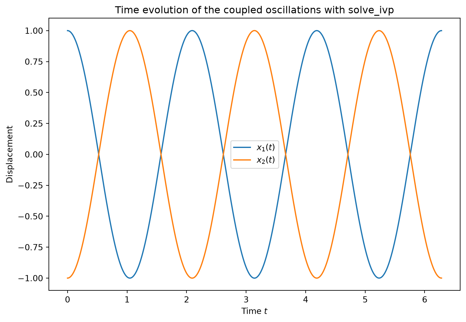
The following code solves this system for $m_1 = m_2 = 1$, $c_1 = c_2 = 1$, and $c_{12} = 4$ (in the code `m1`, `m2`, `c1`, `c2`, `c12`).
The state vector `y` holds the state variables $y_1, \dots, y_4$ under the names `x1`, `x2`, `v1`, `v2`.
The initial conditions $x_1(0) = 1$, $x_2(0) = -1$, and $\dot{x}_1(0) = \dot{x}_2(0) = 0$ excite the antiphase normal mode from @rem-eigenwerte-eigenvektoren.
```{python}
import numpy as np
from scipy.integrate import solve_ivp
import matplotlib.pyplot as plt
from numpy import pi

# Parameters
m1, m2 = 1.0, 1.0  # masses
c1, c2 = 1.0, 1.0  # spring constants of the individual springs
c12 = 4.0  # spring constant of the coupling spring

def dgl_system(t, y, m1, m2, c1, c2, c12):
    x1, x2, v1, v2 = y
    dx1dt = v1
    dx2dt = v2
    dv1dt = -(c1*x1 + c12*(x1-x2)) / m1
    dv2dt = -(c2*x2 + c12*(x2-x1)) / m2
    return [dx1dt, dx2dt, dv1dt, dv2dt]

# Initial conditions: x1(0) = 1, x2(0) = -1, v1(0) = v2(0) = 0
y0 = [1.0, - 1.0, 0.0, 0.0]

# Time span over which the solution is computed
t_span = (0, 2*pi)  # start and end
t_eval = np.linspace(*t_span, 1000)  # time points at which the solution is reported

# Compute the solution
sol = solve_ivp(dgl_system, t_span, y0, args=(m1, m2, c1, c2, c12), t_eval=t_eval)

# Plot the solution
plt.figure(figsize=(9, 6))
plt.plot(sol.t, sol.y[0], label=r'$x_1(t)$')
plt.plot(sol.t, sol.y[1], label=r'$x_2(t)$')
plt.xlabel(r'Time $t$')
plt.ylabel('Displacement')
plt.title('Time evolution of the coupled oscillations with solve_ivp')
plt.legend()
plt.show()
```
:::
::: {#exr-gekoppelt-anfangsbedingungen}
### Changing the Initial Conditions
* Write a function to which different initial conditions can be passed, and use it to investigate the effect of different initial conditions on the system.
* Investigate the behavior of the system for different masses and spring constants of the two springs (e.g., $m_1 \neq m_2$, $c_1 \neq c_2$).
:::