---
jupyter: python3
---
# Numerical Integration of a Differential Equation
Chapter 6 ("Numerical Integration of a Differential Equation") in Part IV of @papu15a gives an introduction to the numerical integration of ODEs.
The symbols used in this chapter are listed in @tbl-symbole-03.
| Symbol | Meaning | Type | Defined in |
|:--|:--|:--|:--|
| $\mathrm{d}$ | Differential ($\mathrm{d}x$, $\frac{\mathrm{d}y}{\mathrm{d}x}$) | Operator | Ch. 02 |
| $\mathrm{e}$ | Euler's number | Constant | @exm-ode-1st-order |
| $f$ | Function; right-hand side of the ODE $y' = f(x,y)$ or $u' = f(t,u)$ | Function | @def-streckenzugverfahren-euler, @eq-ode |
| $g$ | Gravitational acceleration | Constant | @eq-faden |
| $h$ | Step size of an integration scheme; grid spacing $h = 1/(n+1)$ | Scalar | @def-streckenzugverfahren-euler |
| $i$ | Running index (component, row, eigenvalue number, spring number) | Index | Ch. 02 |
| $k$ | Running index (time/iteration step, mode, eigenvalue number) | Index | @def-streckenzugverfahren-euler |
| $k_1, \dots, k_4$ | Increments of the Runge-Kutta method, $k_i = h\,s_i$ | Scalar | @def-rk2, @def-rk4 |
| $l$ | Length of the simple pendulum | Constant | @eq-faden |
| $n$ | Order of an ODE; dimension of a matrix or system; number of steps | Index | Ch. 02, @def-streckenzugverfahren-euler |
| $p$ | Order of consistency, $O(h^p)$ | Index | @def-genauigkeit |
| $s_1, \dots, s_4$; $\bar{s}$ | Slope values of the Runge-Kutta method of order 4; mean slope | Scalar | @fig-rk4 |
| $t$ | Time | Scalar | Ch. 02 |
| $t_k$ | $k$-th time point of the grid; $t_0$ initial time, $t_f$ final time | Scalar | @exm-pendel-euler-matrix |
| $x$ | Independent variable (Ch. 02 §1–4, 03, 06, 08 eigenfunctions) | Scalar | Ch. 02 |
| $x_k, y_k$ | Grid point $x_k = x_0 + kh$ and approximation $y_k \approx y(x_k)$ | Scalar | @def-streckenzugverfahren-euler |
| $y$ | Unknown function $y(x)$ or vector of unknown functions; $y', y'', y^{(n)}$ derivatives | Function | Ch. 02 |
| $y_0$ | Initial value $y(x_0)$ | Scalar | Ch. 02 |
| $y_1, \dots, y_n$ | Components of the state vector $S$ in the reduction of order ($y_1 = y$, $y_2 = y'$, …) or of the solution vector $y$ of a system | Function | @thm-reduktion-ordnung |
| $y_1(k), y_2(k)$ | Approximation of the components $y_1$, $y_2$ of the state vector in step $k$ | Scalar | @exm-pendel-euler-matrix |
| $O(h^p)$ | Landau symbol (order of magnitude of the error) | Operator | @def-genauigkeit |
| $P_0, P_k, Q, R, S$ | Points in the geometric interpretation of the Euler and Runge-Kutta methods | Point | @def-streckenzugverfahren-euler, @fig-rk4 |
| $S$ | State vector $S(t)$; $S_i$ its $i$-th component, $S_0$ initial state | Vector | Ch. 02, @eq-pendel-matrix |
| $\gamma_i$ | Coefficient of a linear combination (weights of the RK2 method; expansion of the starting vector in eigenvectors; basis representation in the eigenspace) | Scalar | @eq-integration |
| $\Delta y_k$ | Increment in step $k$ | Scalar | @tbl-mitttelpunktsmethode-rechenschema |
| $\eta_1, \eta_2$ | Node parameters of the RK2 ansatz (fractions of $h$ in the time and state directions) | Scalar | @eq-integration |
| $\varphi(t)$ | Angle of deflection of the simple pendulum; $\varphi_0$ initial deflection | Function | @eq-faden |
| $y', y'', y^{(n)}$ | First, second, $n$-th derivative with respect to the independent variable | Operator | Ch. 02 |
| $\frac{\partial}{\partial t}$ | Partial derivative | Operator | Ch. 02 |
| $A^{-1}$ | Inverse | Operator | @exm-pendel-euler-matrix |
| local | Line elements $a, b, c, d$, straight line $g$, and coordinates $x_Q, y_Q, x_R, y_R, x_S, y_S$ of the construction in @fig-rk4; intermediate value $y_{h/2}$ of the midpoint method | local | @fig-rk4, @tbl-mitttelpunktsmethode-rechenschema |
: Symbols in Chapter 03 {#tbl-symbole-03}
## Explicit Euler Method (Euler's Polygon Method)
::: {#def-streckenzugverfahren-euler}
#### Explicit Euler Method (Euler's Polygon Method)
Let a first-order ODE
$$
y' = f(x,y)
$$
with the initial point $P_0 = (x_0, y_0)$ be given.
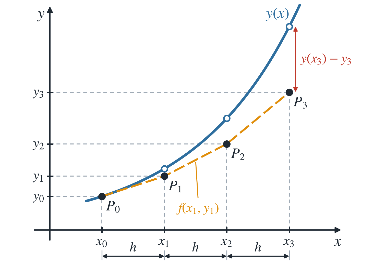
The *explicit Euler method* (*Euler's polygon method*) computes the solution curve $y = y(x)$ point by point at the positions $x_k = x_0 + kh$ with the step size $h$ according to the iteration rule
$$
y(x_k) \approx y_k = y_{k-1} + h f(x_{k-1}, y_{k-1}) \quad (k = 1, 2, \ldots, n),
$$ {#eq-euler-expl-iteration}
see @fig-streckenzugverfahren-euler.
:::
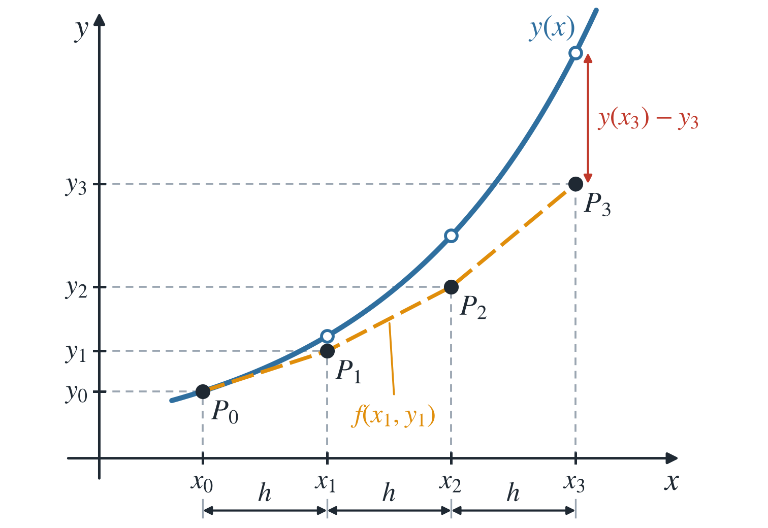{#fig-streckenzugverfahren-euler width=75% fig-alt="Coordinate system with an exponentially increasing exact solution curve and a dashed polygon of three straight segments of equal width h that runs below the curve. The vertices P0 to P3 are marked on the axes with their coordinates x0 to x3 and y0 to y3. A red double arrow shows the growing gap between the exact solution and the approximation at the last step."}
For practical computation, the computational scheme in @tbl-euler-rechenschema is used.
| $k$ | $x$ | $y$ | $h \times f(x,y)$ |
|-----|-----|-----|--------------|
| 0 | $x_0$ | $y_0$ | $h \times f(x_0, y_0)$ |
| 1 | $x_1 = x_0 + h$ | $y_1 = y_0 + h \times f(x_0, y_0)$ | $h \times f(x_1, y_1)$ |
| 2 | $x_2 = x_0 + 2h$ | $y_2 = y_1 + h \times f(x_1, y_1)$ | $h \times f(x_2, y_2)$ |
| $\vdots$ | $\vdots$ | $\vdots$ | $\vdots$ |
| $n$ | $x_n = x_0 + nh$ | $y_n = y_{n-1} + h \times f(x_{n-1}, y_{n-1})$ | $h \times f(x_n, y_n)$ |
: Computational scheme for Euler's method {#tbl-euler-rechenschema}
::: {#exm-euler-1}
#### Euler's Method
We solve the ODE
$$
y' = \frac{\mathrm{d}y}{\mathrm{d}x} = \mathrm{e}^{-x}
$$
with the initial condition $y(0) = -1$ numerically using Euler's method and compare the result with the exact solution $y(x) = -\mathrm{e}^{-x}$.
We use the step size $h = 0.1$ and compute the approximate solution at the points $x_k = 0.1\,k$ for $k = 0, 1, \ldots, 10$, that is, for $x = 0,\ 0.1,\ 0.2,\ \ldots,\ 1$. The right-hand side $f(x,y) = \mathrm{e}^{-x}$ depends on $x$ only. The iteration rule @eq-euler-expl-iteration therefore reads
$$
y_k = y_{k-1} + h\,\mathrm{e}^{-x_{k-1}} \quad (k = 1, 2, \ldots, 10).
$$
We start with $x_0 = 0$ and $y_0 = -1$:
1. $k = 1$: $h f(x_0, y_0) = 0.1 \cdot \mathrm{e}^{0} = 0.1$, so $y_1 = -1 + 0.1 = -0.9$.
2. $k = 2$: $h f(x_1, y_1) = 0.1 \cdot \mathrm{e}^{-0.1} = 0.090484$, so $y_2 = -0.9 + 0.090484 = -0.809516$.
3. $k = 3$: $h f(x_2, y_2) = 0.1 \cdot \mathrm{e}^{-0.2} = 0.081873$, so $y_3 = -0.809516 + 0.081873 = -0.727643$.
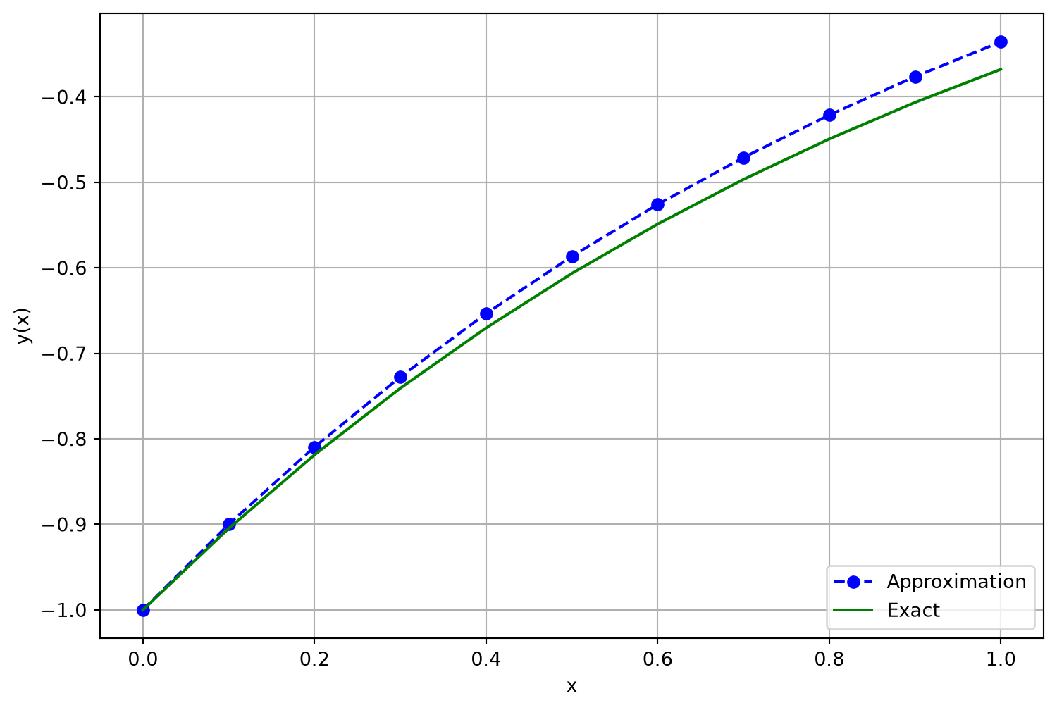
The remaining steps proceed in the same way. @tbl-euler-1 contains the complete computational scheme from @tbl-euler-rechenschema, extended by the exact values $y(x_k) = -\mathrm{e}^{-x_k}$ and the error $y_k - y(x_k)$.
| $k$ | $x_k$ | $y_k$ | $h \times f(x_k,y_k)$ | $y(x_k)$ | $y_k - y(x_k)$ |
|-----|-------|-------|-----------------------|----------|----------------|
| 0 | $0$ | $-1$ | $0.1$ | $-1$ | $0$ |
| 1 | $0.1$ | $-0.9$ | $0.090484$ | $-0.904837$ | $0.004837$ |
| 2 | $0.2$ | $-0.809516$ | $0.081873$ | $-0.818731$ | $0.009214$ |
| 3 | $0.3$ | $-0.727643$ | $0.074082$ | $-0.740818$ | $0.013175$ |
| 4 | $0.4$ | $-0.653561$ | $0.067032$ | $-0.670320$ | $0.016759$ |
| 5 | $0.5$ | $-0.586529$ | $0.060653$ | $-0.606531$ | $0.020001$ |
| 6 | $0.6$ | $-0.525876$ | $0.054881$ | $-0.548812$ | $0.022935$ |
| 7 | $0.7$ | $-0.470995$ | $0.049659$ | $-0.496585$ | $0.025590$ |
| 8 | $0.8$ | $-0.421337$ | $0.044933$ | $-0.449329$ | $0.027992$ |
| 9 | $0.9$ | $-0.376404$ | $0.040657$ | $-0.406570$ | $0.030166$ |
| 10 | $1.0$ | $-0.335747$ | $0.036788$ | $-0.367879$ | $0.032133$ |
: Euler's method for $y' = \mathrm{e}^{-x}$, $y(0) = -1$, with $h = 0.1$ {#tbl-euler-1}
The approximation always lies above the exact solution, and the error grows from step to step. The reason is that the exact solution is concave because $y'' = -\mathrm{e}^{-x} < 0$, and each segment of Euler's method takes the slope at its left endpoint, which exceeds the mean slope over the interval. At $x = 1$ the error is $0.032$, roughly $8.7\,\%$ of the exact value $-0.367879$.
:::
```{python}
import numpy as np

ydot = lambda x, y: np.exp(-x) # ODE
h = 0.1 # step size
x = np.arange(0, 1 + h, h) # computational grid
y0 = -1 # initial value
n = len(x) # number of steps

# Explicit Euler method
y = np.zeros(n)
y[0] = y0
for k in range(0, n - 1):
    y[k + 1] = y[k] + h * ydot(x[k], y[k])
    print(f" k: {k:<2} x: {x[k]:<5.6f} y: {y[k]:<5.6f} h*f: {h*ydot(x[k], y[k]):<5.6f}")
k = n - 1
print(f" k: {k:<2} x: {x[k]:<5.6f} y: {y[k]:<5.6f} h*f: {h*ydot(x[k], y[k]):<5.6f}")
```
```{python}
#| label: fig-euler-1
#| fig-cap: Approximate solution of the differential equation with Euler's method. Step size $h = 0.1$.
import matplotlib.pyplot as plt
%matplotlib inline
plt.figure(figsize = (9, 6))
plt.plot(x, y, 'bo--', label='Approximation')
plt.plot(x, -np.exp(-x), 'g', label='Exact')
plt.xlabel('x')
plt.ylabel('y(x)')
plt.grid()
plt.legend(loc='lower right')
plt.show()
```
In @fig-euler-1 each point is a linear extrapolation of the previous point.
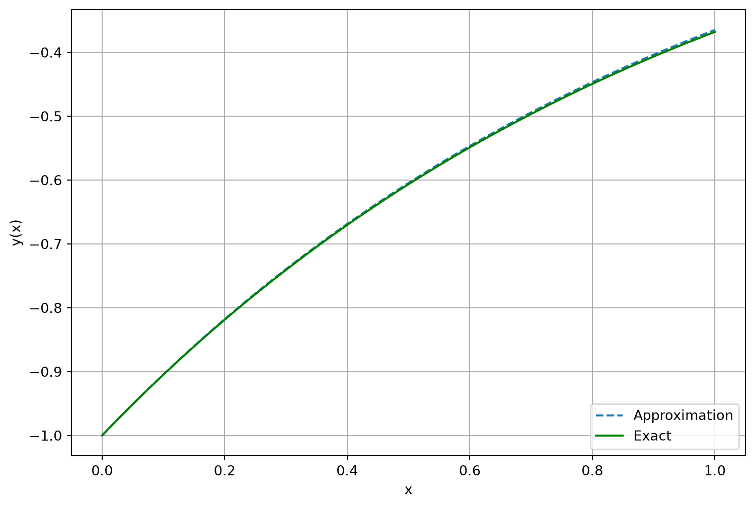
Starting from the initial value, we thus obtain an approximation of the solution on the numerical grid. With $h = 0.01$ the approximation improves, see @fig-euler-2.
```{python}
#| label: fig-euler-2
#| fig-cap: Approximate solution of the differential equation with Euler's method. Step size $h = 0.01$.
import numpy as np

ydot = lambda x, y: np.exp(-x) # ODE
h = 0.01 # step size
x = np.arange(0, 1 + h, h) # computational grid
y0 = -1 # initial value
n = len(x) # number of steps

# Explicit Euler method
y = np.zeros(n)
y[0] = y0
for k in range(0, n - 1):
    y[k + 1] = y[k] + h * ydot(x[k], y[k])

import matplotlib.pyplot as plt
%matplotlib inline
plt.figure(figsize = (9, 6))
plt.plot(x, y, '--', label='Approximation')
plt.plot(x, -np.exp(-x), 'g', label='Exact')
plt.xlabel('x')
plt.ylabel('y(x)')
plt.grid()
plt.legend(loc='lower right')
plt.show()
```
The method is called explicit because $y_{k+1}$ is computed solely from the already known values $x_k$ and $y_k$.
## Implicit Euler Method
The implicit Euler method differs from the explicit (forward) Euler method in that the function $f$ is evaluated at the end point of the step rather than at the starting point.
::: {#def-implizit-euler}
#### Implicit Euler Method
Let the initial value problem
$$
y' = f(x,y), \quad y(x_0) = y_0,
$$
be given with a step size $h > 0$ and the nodes $x_k = x_0 + kh$, $k = 0, 1, \dots$
The *implicit Euler method* computes the approximations $y_k$ according to the iteration rule
$$
y_{k+1} = y_k + hf(x_{k+1}, y_{k+1}), \quad k = 0, 1, \dots
$$ {#eq-euler-impl-iteration}
:::
The value $f(x_{k+1}, y_{k+1})$ is not given explicitly, because $y_{k+1}$ appears on both sides of the equation.
The equation therefore has to be solved for $y_{k+1}$ in every step.
The explicit method does not need this computation, because its rule is already solved for $y_{k+1}$.
The values $y_k$ approximate the values $y(x_k)$ of the exact solution of the initial value problem. The smaller the step size $h$, the higher the computational cost and the better the approximation.
## Trapezoidal Method
Before showing how to solve the implicit Euler formula, we introduce another implicit formula, the trapezoidal formula. It is the average of the explicit and the implicit Euler formulas.
::: {#def-trapez}
#### Trapezoidal Method
The *trapezoidal method* computes the next point in each case according to the iteration rule
$$
y_{k+1} = y_k + \frac{h}{2}\left( f(x_k, y_k) + f(x_{k+1}, y_{k+1}) \right).
$$ {#eq-euler-trapez-iteration}
:::
The method can be read as a predictor-corrector scheme. First, the explicit Euler method yields a preliminary value for $y_{k+1}$ (predictor step). This value is used to compute the slope at the end of the interval. The average of the slopes at the beginning and at the end of the interval then determines the final value $y_{k+1}$.
## Simple Pendulum: Euler Methods in Matrix Form
To show how the implicit schemes (@eq-euler-impl-iteration and @eq-euler-trapez-iteration) are solved, we consider the pendulum equation, which was reduced to a first-order system in @eq-reduktion-fadenpendel-matrix.
With the state vector $S(t) = (y_1(t), y_2(t))^T = (\varphi(t), \dot{\varphi}(t))^T$ it reads
$$
\frac{\mathrm{d}S(t)}{\mathrm{d}t} = f(t, S(t)) =
\begin{pmatrix}
0 & 1\\
-\frac{g}{l} & 0\\
\end{pmatrix} S(t).
$$ {#eq-pendel-matrix}
::: {#exm-pendel-euler-matrix}
#### Euler and Trapezoidal Methods for the Simple Pendulum
We consider the time points $t_k = t_0 + kh$ and write $y_1(k)$ and $y_2(k)$ for the approximations of the components $y_1(t_k)$ and $y_2(t_k)$ in step $k$.
Substituting @eq-pendel-matrix into the explicit Euler formula @eq-euler-expl-iteration
$$
y_{k+1} = y_{k} + h f(x_{k}, y_{k})
$$
we obtain
$$
\begin{pmatrix}
y_1(k+1)\\
y_2(k+1)\\
\end{pmatrix} =
\begin{pmatrix}
y_1(k)\\
y_2(k)\\
\end{pmatrix} +
h
\begin{pmatrix}
0 & 1\\
-\frac{g}{l} & 0\\
\end{pmatrix}
\begin{pmatrix}
y_1(k)\\
y_2(k)\\
\end{pmatrix} =
\begin{pmatrix}
1 & h\\
-\frac{gh}{l} & 1\\
\end{pmatrix}
\begin{pmatrix}
y_1(k)\\
y_2(k)\\
\end{pmatrix}.
$$
Substituting @eq-pendel-matrix into the implicit Euler formula @eq-euler-impl-iteration
$$
y_{k+1} = y_k + hf(x_{k+1}, y_{k+1})
$$
yields
$$
\begin{pmatrix}
y_1(k+1)\\
y_2(k+1)\\
\end{pmatrix} =
\begin{pmatrix}
y_1(k)\\
y_2(k)\\
\end{pmatrix} +
h
\begin{pmatrix}
0 & 1\\
-\frac{g}{l} & 0\\
\end{pmatrix}
\begin{pmatrix}
y_1(k+1)\\
y_2(k+1)\\
\end{pmatrix}
$$
and hence
$$
\begin{pmatrix}
1 & -h \\
\frac{gh}{l} & 1
\end{pmatrix}
\begin{pmatrix}
y_1(k+1)\\
y_2(k+1)\\
\end{pmatrix}
=
\begin{pmatrix}
y_1(k)\\
y_2(k)\\
\end{pmatrix}.
$$
Rearranging (matrix inversion) yields
$$
\begin{pmatrix}
y_1(k+1)\\
y_2(k+1)\\
\end{pmatrix}
=
\begin{pmatrix}
1 & -h \\
\frac{gh}{l} & 1
\end{pmatrix}^{-1}
\begin{pmatrix}
y_1(k)\\
y_2(k)\\
\end{pmatrix}.
$$
Substituting into the trapezoidal formula @eq-euler-trapez-iteration
$$
y_{k+1} = y_k + \frac{h}{2}\left( f(x_k, y_k) + f(x_{k+1}, y_{k+1}) \right)
$$
we obtain
$$
\begin{pmatrix}
y_1(k+1)\\
y_2(k+1)\\
\end{pmatrix} =
\begin{pmatrix}
y_1(k)\\
y_2(k)\\
\end{pmatrix} +
\frac{h}{2}
\left\{
\begin{pmatrix}
0 & 1\\
-\frac{g}{l} & 0\\
\end{pmatrix}
\begin{pmatrix}
y_1(k)\\
y_2(k)\\
\end{pmatrix} +
\begin{pmatrix}
0 & 1\\
-\frac{g}{l} & 0\\
\end{pmatrix}
\begin{pmatrix}
y_1(k+1)\\
y_2(k+1)\\
\end{pmatrix}
\right\}
$$
and from this
$$
\begin{pmatrix}
1 & -\frac{h}{2} \\
\frac{gh}{2l} & 1
\end{pmatrix}
\begin{pmatrix}
y_1(k+1)\\
y_2(k+1)\\
\end{pmatrix} =
\begin{pmatrix}
1 & \frac{h}{2} \\
-\frac{gh}{2l} & 1
\end{pmatrix}
\begin{pmatrix}
y_1(k)\\
y_2(k)\\
\end{pmatrix}.
$$
Solving for $y_{k+1}$ yields for the trapezoidal formula
$$
\begin{pmatrix}
y_1(k+1)\\
y_2(k+1)\\
\end{pmatrix} =
\begin{pmatrix}
1 & -\frac{h}{2} \\
\frac{gh}{2l} & 1
\end{pmatrix}^{-1}
\begin{pmatrix}
1 & \frac{h}{2} \\
-\frac{gh}{2l} & 1
\end{pmatrix}
\begin{pmatrix}
y_1(k)\\
y_2(k)\\
\end{pmatrix}.
$$
:::
These equations solve the initial value problem, because the next state $S(t_{k+1})$ can be computed from every state $S(t_k)$. In general, this is possible whenever the ODE is linear.
## Numerical Error and Instability
For integration schemes for ODEs, two questions are central: accuracy and stability.
::: {#def-genauigkeit}
#### Accuracy
The *accuracy* of an integration scheme describes how well it approximates the (usually unknown) exact solution as a function of the step size $h$. It is stated in $O$-notation: a scheme has order $p$ if its error behaves like $O(h^p)$ for $h \to 0$.
:::
::: {#def-stabilitaet}
#### Stability
The *stability* of an integration scheme is its ability to keep the error from growing while integrating forward in time. If the error does not grow, the scheme is stable; otherwise it is unstable. A scheme that is stable only for certain step sizes $h$ is also referred to as unstable.
:::
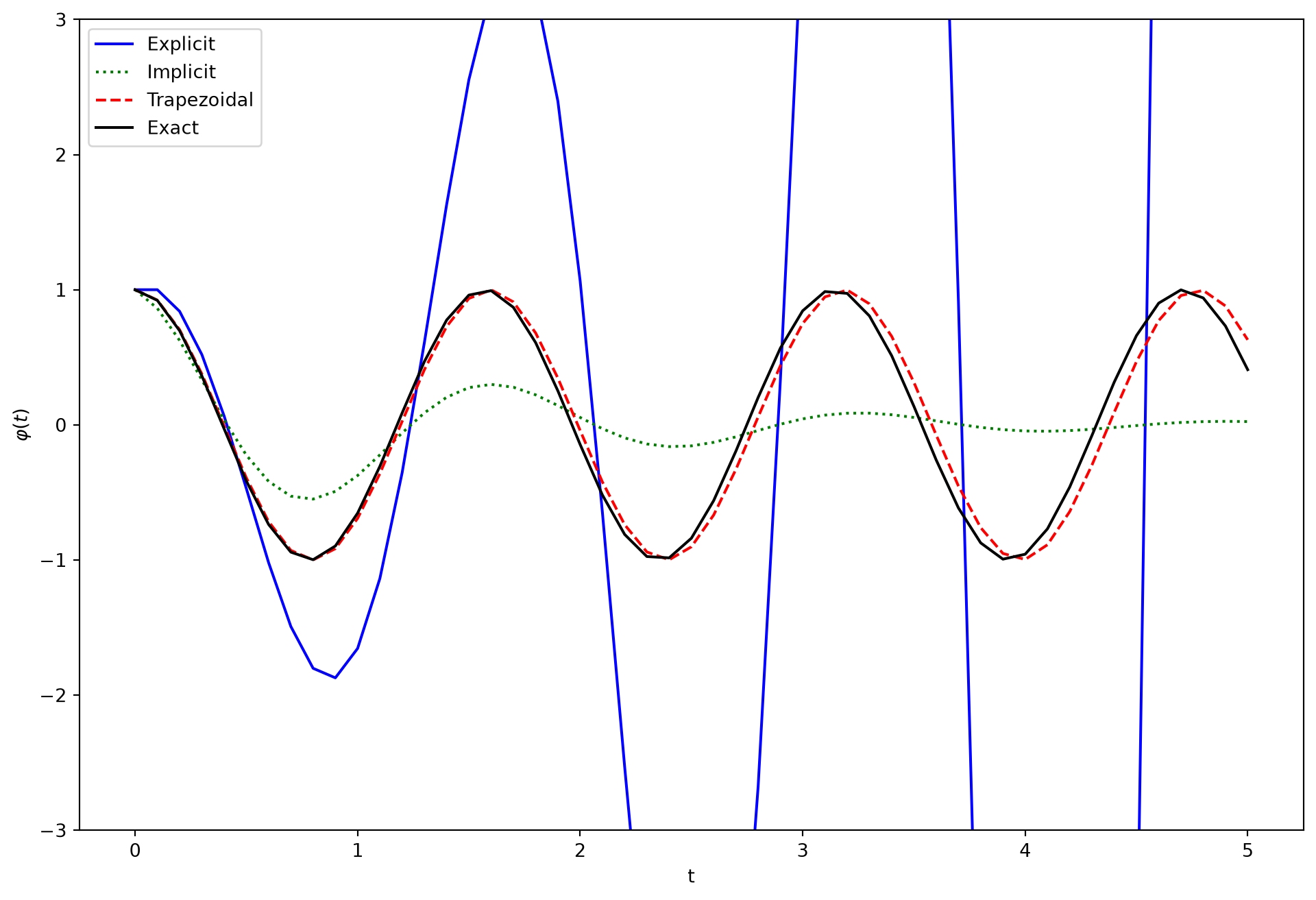
To illustrate stability problems, in @exm-euler-2 we solve the pendulum equation numerically using the explicit Euler method, the implicit Euler method, and the trapezoidal rule.
::: {#exm-euler-2}
#### Programming the Euler Methods
We solve the pendulum equation @eq-pendel-matrix over the time interval $[0,\,5]$ with the step size $h = 0.1$ and the initial state
$$
S_0 = \begin{pmatrix} 1 \\ 0 \end{pmatrix}
$$
using the explicit Euler method, the implicit Euler method, and the trapezoidal rule.
For the model parameters we use $\sqrt{g/l} = 4$ (`w` in the code).
:::
```{python}
import numpy as np
from numpy.linalg import inv
import matplotlib.pyplot as plt

%matplotlib inline
```
```{python}
# define step size
h = 0.1
# define numerical grid
t = np.arange(0, 5.1, h)
# oscillation freq. of pendulum
w = 4
s0 = np.array([[1], [0]])

m_e = np.array([[1, h],
               [-w**2*h, 1]])
m_i = inv(np.array([[1, -h],
               [w**2*h, 1]]))
m_t = np.dot(inv(np.array([[1, -h/2],
    [w**2*h/2,1]])), np.array(
      [[1,h/2], [-w**2*h/2, 1]]))

s_e = np.zeros((len(t), 2))
s_i = np.zeros((len(t), 2))
s_t = np.zeros((len(t), 2))

# do integrations
s_e[0, :] = s0.T
s_i[0, :] = s0.T
s_t[0, :] = s0.T

for j in range(0, len(t)-1):
    s_e[j+1, :] = np.dot(m_e,s_e[j, :])
    s_i[j+1, :] = np.dot(m_i,s_i[j, :])
    s_t[j+1, :] = np.dot(m_t,s_t[j, :])
```
```{python}
#| label: fig-euler-winkel
#| fig-cap: Comparison of the numerical solutions for the angle of deflection $\varphi(t)$ of the pendulum with the explicit, implicit, and trapezoidal rules.
plt.figure(figsize = (12, 8))
plt.plot(t,s_e[:,0],'b-')
plt.plot(t,s_i[:,0],'g:')
plt.plot(t,s_t[:,0],'r--')
plt.plot(t, np.cos(w*t), 'k')
plt.ylim([-3, 3])
plt.xlabel('t')
plt.ylabel(r'$\varphi(t)$')
plt.legend(['Explicit', 'Implicit', \
            'Trapezoidal', 'Exact'])
plt.show()
```
@fig-euler-winkel shows the angle $\varphi$ over the time $t$. The exact solution is a pure cosine wave. The explicit Euler method is clearly unstable. The solution of the implicit Euler method decays exponentially, which is not correct. The trapezoidal rule captures the solution correctly, although with a small phase shift that increases with time.
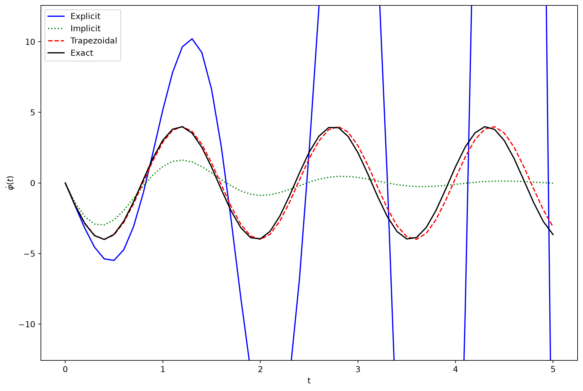
@fig-euler-winkelgeschwindigkeit shows the angular velocity $\dot{\varphi}(t)$ of the pendulum.
```{python}
# define step size
h = 0.1
# define numerical grid
t = np.arange(0, 5.1, h)
# oscillation freq. of pendulum
w = 4
s0 = np.array([[1], [0]])

m_e = np.array([[1, h],
               [-w**2*h, 1]])
m_i = inv(np.array([[1, -h],
               [w**2*h, 1]]))
m_t = np.dot(inv(np.array([[1, -h/2],
    [w**2*h/2,1]])), np.array(
      [[1,h/2], [-w**2*h/2, 1]]))

s_e = np.zeros((len(t), 2))
s_i = np.zeros((len(t), 2))
s_t = np.zeros((len(t), 2))

s_e[0, :] = s0.T
s_i[0, :] = s0.T
s_t[0, :] = s0.T
```
```{python}
#| label: fig-euler-winkelgeschwindigkeit
#| fig-cap: Comparison of the numerical solutions for the angular velocity $\dot{\varphi}(t)$ of the pendulum with the explicit, implicit, and trapezoidal rules.
for j in range(0, len(t)-1):
    s_e[j+1, :] = np.dot(m_e,s_e[j, :])
    s_i[j+1, :] = np.dot(m_i,s_i[j, :])
    s_t[j+1, :] = np.dot(m_t,s_t[j, :])

plt.figure(figsize = (12, 8))
plt.plot(t,s_e[:,1],'b-')
plt.plot(t,s_i[:,1],'g:')
plt.plot(t,s_t[:,1],'r--')
plt.plot(t, -w*np.sin(w*t), 'k')
plt.ylim([-4*np.pi, 4*np.pi])
plt.xlabel('t')
plt.ylabel(r'$\dot{\varphi}(t)$')
plt.legend(['Explicit', 'Implicit', \
            'Trapezoidal', 'Exact'])
plt.show()
```
## Runge-Kutta Methods
Runge-Kutta (RK) methods are among the most widely used methods for solving ODEs.
They estimate the slope of the solution given by the ODE at several points within one time step. These estimates yield the next value without an explicit correction phase.
### The Midpoint Method
More sophisticated methods achieve a higher order and thus more accuracy.
One possibility is additional function evaluations, as the midpoint method in @def-mittelpunktsmethode shows.
::: {#def-mittelpunktsmethode}
#### The Midpoint Method
The *midpoint method* computes the next point in each case according to the iteration rule
$$
y_{k+1} = y_k + h f
\left(
x_k + \frac{1}{2} h, y_k + \frac{1}{2} h f(x_k, y_k)
\right).
$$
:::
The midpoint method improves on the explicit Euler method by evaluating the slope not only at the starting point but also at the middle of the interval.
In its first step, it uses the slope at the starting point to predict the solution value halfway between $x_k$ and $x_{k+1}$:
$$
y\left( x_k + \frac{h}{2} \right) = y(x_k) + \frac{h}{2}f(x_k, y(x_k)).
$$
The slope at this point then determines the value at the end of the interval:
$$
y(x_{k+1}) = y(x_k) + h f\left(x_k + \frac{h}{2}, y\left(x_k + \frac{h}{2}\right)\right).
$$
::: {#exm-mittelpunktsmethode}
#### Midpoint Method
For the initial value problem
$$
y' = f(x,y) = y + \mathrm{e}^x, \quad y(0) = 1,
$$
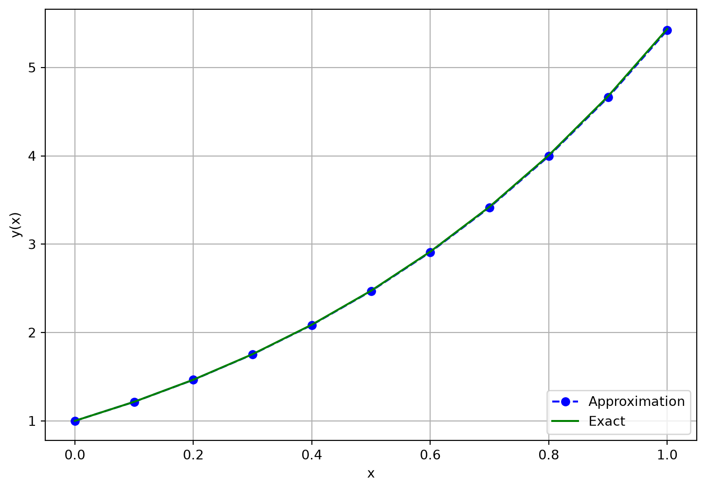
with the exact solution $y(x) = (x+1)\, \mathrm{e}^x$, the midpoint method with step size $h = 0.1$ can be carried out using the computational scheme in @tbl-mitttelpunktsmethode-rechenschema.
| $k$ | $x$ | $y$ | $y_{\frac{h}{2}} = y + \frac{h}{2} f(x,y)$ | $\Delta y = h \times f(x + \frac{h}{2}, y_{\frac{h}{2}})$ |
|-|-|----|------|------|
| 0 | $x_0$ | $y_0$ | $y_{\frac{h}{2},0} = y_0 + \frac{h}{2} \times f(x_0, y_0)$ | $\Delta y_0 = h \times f(x_0 + \frac{h}{2}, y_{\frac{h}{2},0})$ |
| 1 | $x_1 = x_0 + h$ | $y_1 = y_0 + \Delta y_0$ | $y_{\frac{h}{2},1} = y_1 + \frac{h}{2} \times f(x_1, y_1)$ | $\Delta y_1 = h \times f(x_1 + \frac{h}{2}, y_{\frac{h}{2},1})$ |
| 2 | $x_2 = x_1 + h$ | $y_2 = y_1 + \Delta y_1$ | $y_{\frac{h}{2},2} = y_2 + \frac{h}{2} \times f(x_2, y_2)$ | $\Delta y_2 = h \times f(x_2 + \frac{h}{2}, y_{\frac{h}{2},2})$ |
| $\vdots$ | $\vdots$ | $\vdots$ | $\vdots$ | $\vdots$ |
| $n$ | $x_n = x_0 + nh$ | $y_n = y_{n-1} + \Delta y_{n-1}$ | | |
: Computational scheme for the midpoint method {#tbl-mitttelpunktsmethode-rechenschema}
:::
An implementation of the midpoint method for @exm-mittelpunktsmethode in Python reads:
```{python}
import numpy as np

ydot = lambda x, y: y + np.exp(x) # ODE
h = 0.1 # step size
h2 = h/2
x = np.arange(0, 1 + h, h) # computational grid
y0 = 1 # initial value
n = len(x) # number of steps

# Midpoint method
y = np.zeros(n)
y2 = np.zeros(n)
y[0] = y0
for k in range(0, n - 1):
    y2[k] = y[k] + h2 * ydot(x[k], y[k])
    y[k + 1] = y[k] + h * ydot(x[k] + h2, y2[k])
    print(f" k: {k:<2} x: {x[k]:<5.1f} y: {y[k]:<5.8f} y2: {y2[k]:<5.8f} h*f: {h*ydot(x[k] + h2, y2[k]):<5.8f}")
k = n - 1
print(f" k: {k:<2} x: {x[k]:<5.1f} y: {y[k]:<5.8f} y2: {y2[k]:<5.8f} h*f: {h*ydot(x[k] + h2, y2[k]):<5.8f}")
```
```{python}
#| label: fig-mittelpunktsmethode
#| fig-cap: Approximate solution of the differential equation $y'=y+\mathrm{e}^x$ with the midpoint method. Step size $h = 0.1$.
import matplotlib.pyplot as plt
%matplotlib inline
plt.figure(figsize = (9, 6))
plt.plot(x, y, 'bo--', label='Approximation')
plt.plot(x, (x+1)*np.exp(x), 'g', label='Exact')
plt.xlabel('x')
plt.ylabel('y(x)')
plt.grid()
plt.legend(loc='lower right')
plt.show()
```
The midpoint method belongs to the family of Runge-Kutta methods; it is a second-order Runge-Kutta method.
### Derivation of the Runge-Kutta Methods
Euler's method approximates the state $S$ with the first two terms of the Taylor series, that is, linearly:
$$
S(t_{k+1}) = S(t_k + h) = S(t_k) + h \cdot S'(t_k).
$$
Further terms of the Taylor series improve the accuracy of the numerical integration considerably:
$$
S(t_{k+1}) = S(t_k + h) = S(t_k) + S'(t_k)h + \frac{1}{2!}S''(t_k)h^2 + \cdots + \frac{1}{n!}S^{(n)}(t_k)h^n.
$$ {#eq-taylor}
This would require deriving the expressions for $S''(t_k), S'''(t_k), \dots, S^{(n)}(t_k)$.
The RK methods avoid this additional work. They are based on truncated Taylor series but do not require higher derivatives.
#### Second-Order Runge-Kutta Method {#sec-rk2}
We derive the second-order Runge-Kutta method.
Let
$$
\frac{\mathrm{d}S(t)}{\mathrm{d}t} = f(t,S(t)).
$$ {#eq-ode}
We assume an integration formula of the form
$$
S(t + h) = S(t) + \gamma_1 f(t, S(t))h + \gamma_2 f\big(t+\eta_1 h, S(t)+\eta_2 hf(t, S(t))\big)h
$$ {#eq-integration}
that requires no derivatives of $S(t)$ beyond first order.
Derivatives of second and higher order arise from combinations of $f(t, S(t))$ and $f\big(t+\eta_1 h, S(t)+\eta_2 hf(t, S(t))\big)$.
We determine the parameters $\gamma_1, \gamma_2, \eta_1, \eta_2$ by comparing @eq-integration with the second-order Taylor series.
::: {#prp-rk2-ordnungsbedingungen}
#### Order Conditions of the Second-Order Runge-Kutta Ansatz
For every right-hand side $f$, the integration formula @eq-integration agrees with the Taylor series @eq-taylor up to terms of order $h^3$ if and only if
$$
\gamma_1 + \gamma_2 = 1, \quad \gamma_2\eta_1=\frac{1}{2}, \quad \gamma_2\eta_2=\frac{1}{2}.
$$ {#eq-result}
:::
::: {.proof}
The second-order Taylor series reads
$$
S(t + h) = S(t) + S'(t)h + \frac{1}{2!}S''(t)h^2 = S(t) + f(t, S(t))h + \frac{1}{2!}f'(t, S(t))h^2.
$$ {#eq-matching}
Because of @eq-ode, the time derivative of $f$ is
$$
f'(t, S(t)) = \frac{\partial f}{\partial t} + \frac{\partial f}{\partial S}\frac{\mathrm{d}S}{\mathrm{d}t} = \frac{\partial f}{\partial t} + \frac{\partial f}{\partial S}f.
$$
Hence @eq-matching can be written as
$$
S(t + h) = S + fh + \frac{1}{2!}\Big(\frac{\partial f}{\partial t} + \frac{\partial f}{\partial S}f\Big)h^2.
$$ {#eq-rewrite-matching}
We expand the last term in @eq-integration with the Taylor series in several variables:
$$
f(t+\eta_1 h, S+\eta_2 hf) \approx f + \frac{\partial f}{\partial t}\eta_1 h + \eta_2 h\frac{\partial f}{\partial S}f.
$$
Hence @eq-integration becomes
$$
S(t + h) = S + (\gamma_1+\gamma_2)fh + (\gamma_2\eta_1)\frac{\partial f}{\partial t}h^2 + (\gamma_2\eta_2)\frac{\partial f}{\partial S}fh^2.
$$ {#eq-rewrite-integration}
Comparing the coefficients of @eq-rewrite-matching and @eq-rewrite-integration yields @eq-result.
:::
Since @eq-result has four unknowns and only three equations, we can choose one parameter freely and determine the remaining ones from it. A popular choice is
$$
\gamma_1 =\frac{1}{2}, \quad \gamma_2 =\frac{1}{2}, \quad \eta_1 =1, \quad \eta_2=1.
$$
::: {#def-rk2}
#### Second-Order Runge-Kutta Method
With parameters $\gamma_1, \gamma_2, \eta_1, \eta_2$ that satisfy @eq-result and the increments
$$
\begin{aligned}
k_1 &= h f(t_k, S(t_k)),\\
k_2 &= h f\left(t_k + \eta_1 h, S(t_k) + \eta_2 k_1\right)
\end{aligned}
$$
the *second-order Runge-Kutta method* computes the next state as
$$
S(t_{k+1}) \approx S(t_k) + \gamma_1 k_1 + \gamma_2 k_2.
$$
For $\gamma_1 = \gamma_2 = \frac{1}{2}$ and $\eta_1 = \eta_2 = 1$, this gives $S(t_{k+1}) \approx S(t_k) + \frac{1}{2}(k_1 + k_2)$.
:::
#### Runge-Kutta Method of Order 4
A classical method for integrating ODEs with high accuracy is the fourth-order Runge-Kutta method (RK4). It can be derived from the Taylor series similarly to @sec-rk2.
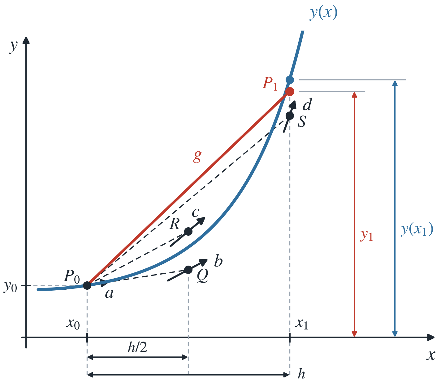
Here we motivate it geometrically, see @fig-rk4.
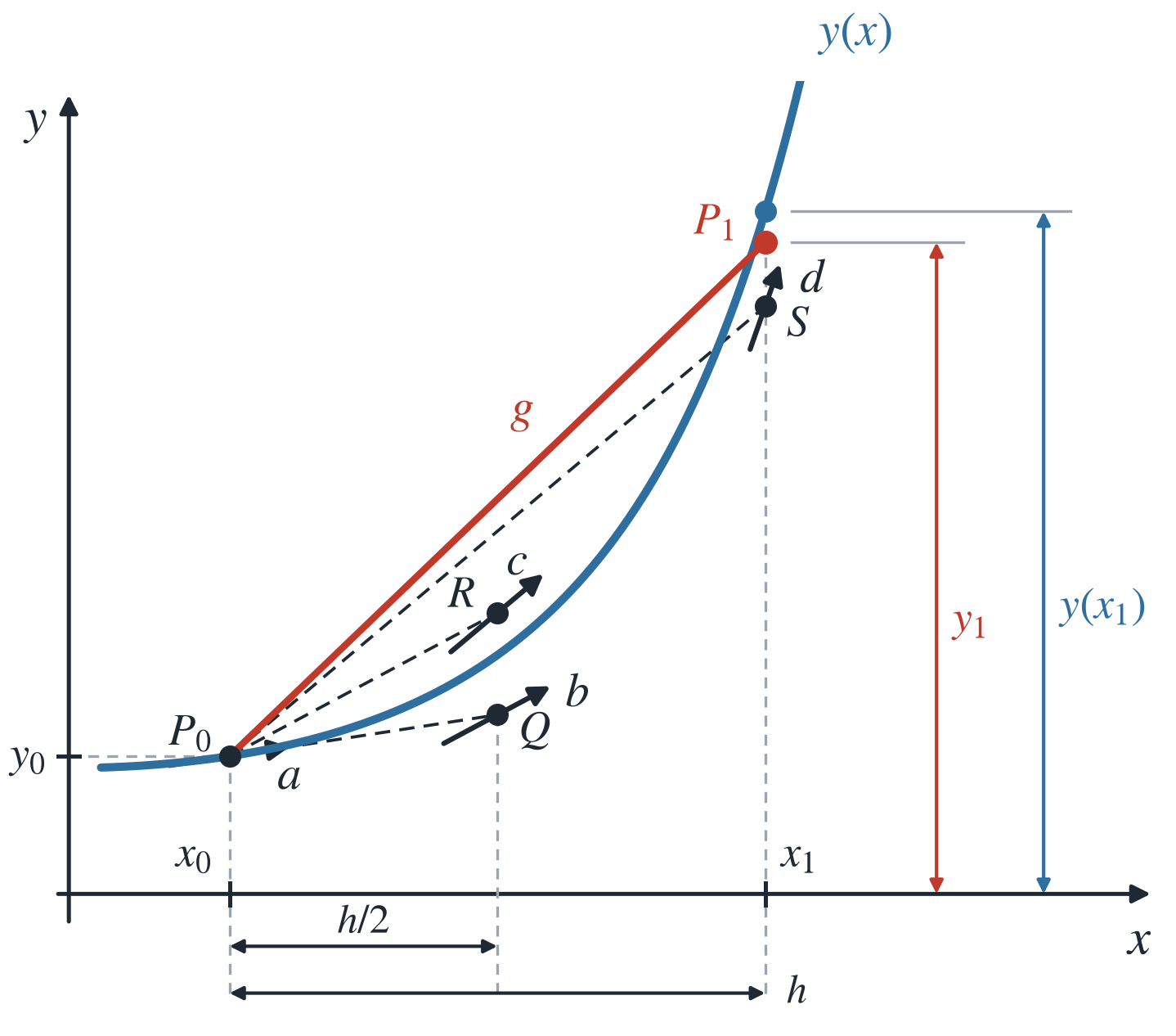{#fig-rk4 width=70% fig-alt="A convex, increasing exact solution curve passes through the initial point P0. Dashed straight lines lead from P0 to the auxiliary points Q and R at the middle of the interval and S at its end; short arrows at these points indicate the respective slope. A red straight line g leads from P0 to the end point P1, which lies just below the point of the exact solution at x1; on the right, y1 and y(x1) are drawn as dimension arrows."}
Starting from the initial point $P_0$, we move along a straight line $g$ with the mean slope $\bar{s}$ to the end of the interval $x_1 = x_0 + h$. The ordinate $y_1$ of the end point $P_1$ reached in this way is an approximation of the sought solution $y(x_1)$. The mean slope is determined from four slope values, one at each of the two boundary points of the interval and two at the middle of the interval. The values at the middle of the interval enter the mean slope $\bar{s}$ with a larger weight.
::: {.callout-tip}
#### Summary: Runge-Kutta Method of Order 4
1. From $P_0$ with slope $s_1$ by $h/2$ to $Q$; determine the slope $s_2$ there.
2. From $P_0$ with slope $s_2$ by $h/2$ to $R$; determine the slope $s_3$ there.
3. From $P_0$ with slope $s_3$ by $h$ to $S$; determine the slope $s_4$ there.
4. From $P_0$ with the mean slope $\bar{s} = \frac{1}{6}(s_1 + 2s_2 + 2s_3 + s_4)$ by $h$ to $P_1$.
@papu15a computes with the increments $k_i = h\,s_i$ instead of the slopes $s_i$.
:::
The first slope $s_1 = f(x_0, y_0)$ is the slope of the tangent to the solution curve at the initial point $P_0$ (line element $a$).
Along this tangent we move from $P_0$ to the middle of the interval and reach the point $Q$ with the coordinates
$$
x_Q = x_0 + \frac{h}{2} \qquad \text{and} \qquad y_Q= y_0 + \frac{1}{2} h \times f(x_0, y_0) = y_0 + \frac{k_1}{2}, \qquad k_1 = h \times f(x_0, y_0).
$$
The solution curve through $Q$ has the line element $b$ there with the slope
$$
s_2 = f\left(x_0 + \frac{h}{2}, y_0 + \frac{k_1}{2}\right).
$$
Parallel to the line element $b$, we again move from $P_0$ to the middle of the interval and reach the point $R$ with the coordinates
$$
x_R = x_0 + \frac{h}{2} \qquad \text{and} \qquad y_R = y_0 + \frac{1}{2}h \times s_2 = y_0 + \frac{k_2}{2}, \qquad k_2 = h \times s_2.
$$
The solution curve through $R$ has the line element $c$ there with the slope
$$
s_3 = f\left(x_0 + \frac{h}{2}, y_0 + \frac{k_2}{2}\right).
$$
Parallel to the line element $c$, we move from $P_0$ to the end of the interval and reach the point $S$ with the coordinates
$$
x_S = x_0 + h \qquad \text{and} \qquad y_S = y_0 + h \times s_3 = y_0 + k_3, \qquad k_3 = h \times s_3.
$$
The solution curve through $S$ has the line element $d$ there with the slope
$$
s_4 = f(x_0 + h, y_0 + k_3).
$$
The slope of the straight line $g$ from the initial point $P_0$ to the end point $P_1$ is the weighted average of the four slope values:
$$
\bar{s} = \frac{1}{6}(s_1 + 2s_2 + 2s_3 + s_4).
$$
::: {#def-rk4}
#### Runge-Kutta Method of Order 4
Let a first-order ODE
$$
y' = f(x,y)
$$
be given with the initial point $P_0 = (x_0, y_0)$, the step size $h = (x_n - x_0)/n$, and the nodes $x_i = x_{i-1} + h$.
The *Runge-Kutta method of order 4* computes the approximations $y_i \approx y(x_i)$ according to the rule
$$
\begin{aligned}
k_1 &= h f(x_{i-1}, y_{i-1}), \\
k_2 &= h f\left(x_{i-1} + \frac{h}{2}, y_{i-1} + \frac{k_1}{2}\right), \\
k_3 &= h f\left(x_{i-1} + \frac{h}{2}, y_{i-1} + \frac{k_2}{2}\right), \\
k_4 &= h f(x_{i-1} + h, y_{i-1} + k_3), \\
y_i &= y_{i-1} + \frac{1}{6} (k_1 + 2 k_2 + 2 k_3 + k_4).
\end{aligned}
$$
:::
Unlike Euler's polygon method, the RK4 method uses a mean slope value $\bar{s}$ for the slope of the substitute straight line. It takes into account the slope behavior of the solution curve at the two boundary points and at the middle of the interval with different weights.
The polygon method, in contrast, uses only the slope $s_1 = f(x_0, y_0)$ at the initial point $P_0$.