10 Models for Vibration Analysis
Strehlau (2011) uses a model of a cyclically symmetric structure consisting of individual masses to understand the basic vibration behavior of blisks, see Figure 10.1.
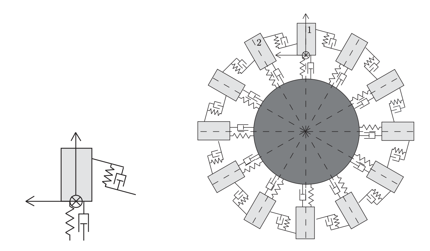
Table 10.1 summarizes the symbols used in this chapter.
| Symbol | Meaning | Type | Defined in |
|---|---|---|---|
| \(c\) | Spring constant | Constant | Theorem 2.7 |
| \(\mathrm{e}\) | Euler’s number | Constant | Example 2.1 |
| \(j\) | Running index (row/column, mass, blade); italic, as distinct from the imaginary unit \(\mathrm{j}\) | Index | Definition 10.1 |
| \(\mathrm{j}\) | Imaginary unit, \(\mathrm{j}^2 = -1\) | Constant | Equation 2.5 |
| \(k\) | Running index (time/iteration step, mode, eigenvalue number) | Index | Definition 3.1 |
| \(m\) | Mass | Constant | Theorem 2.6 |
| \(q, q_j\) | Displacement vector of the oscillator chain; \(q_j\) displacement of element \(j\) | Vector | Equation 10.1 |
| \(\hat{q}, \hat{q}_k\) | Amplitude vector in the ansatz \(q = \hat{q}\,\mathrm{e}^{\lambda t}\); \(\hat{q}_k\) mode shape (eigenvector) of mode \(k\) | Vector | Proposition 10.2 |
| \(t\) | Time | Scalar | Figure 2.2 |
| \(A_k, B_k\) | Coefficients of the real modal solution, \(q(t) = \sum (A_k\cos\omega_k t + B_k \sin\omega_k t)\hat{q}_k\); \(A_0, B_0\) rigid-body component | Scalar | Equation 10.4 |
| \(C_n\) | Circulant matrix (\(-1, 2, -1\) cyclic); \(C_N\) for the ring of \(N\) masses | Matrix | Section 8.1 |
| \(\underline{C}_k\) | Complex coefficient of the modal solution, \(\underline{C}_k = \tfrac12(A_k + \mathrm{j}B_k)\); conjugate \(\overline{\underline{C}}_k\) | Scalar | Equation 10.3 |
| \(D\) | Damping matrix | Matrix | Section 10.1 |
| \(E\) | Identity matrix | Matrix | Definition 5.1 |
| \(G\) | Matrix of the gyroscopic forces (gyroscopic matrix) | Matrix | Section 10.1 |
| \(K\) | Stiffness matrix, \(K = A^TCA\); here \(K = c\,C_N\) | Matrix | Definition 8.5, Equation 10.2 |
| \(K_{ij}\) | Element of the matrix \(K\) in row \(i\), column \(j\) | Scalar | Equation 10.2 |
| \(M\) | Mass matrix, \(M = \operatorname{diag}(m_1, \dots, m_n)\); here \(M = mE\) | Matrix | Definition 8.5 |
| \(N\) | Number of masses, springs, or blades (ring) | Index | Definition 10.1 |
| \(\zeta\) | \(n\)-th root of unity, \(\zeta = \mathrm{e}^{2\pi\mathrm{j}/n}\); \(\overline{\zeta}\) conjugate | Scalar | Section 8.1 |
| \(\lambda\) | Eigenvalue or root of the characteristic equation (exponent in the ansatz \(\mathrm{e}^{\lambda t}\)); \(\lambda_{k\pm} = \pm\mathrm{j}\omega_k\) | Scalar | Definition 5.1 |
| \(\mu_k\) | Eigenvalue of \(C_N\), \(\mu_k = 4\sin^2(\pi k/N)\) | Scalar | Proposition 10.1 |
| \(\pi\) | The number pi | Constant | – |
| \(\varphi_{\mathrm{KD}}\) | Inter-blade phase angle, \(\varphi_{\mathrm{KD}} = 2\pi\,\mathrm{KD}/N\) | Scalar | Definition 10.2 |
| \(\omega_k\) | Natural angular frequency of the \(k\)-th normal mode; it vanishes for \(k = 0\) (never written as \(\omega_0\)) | Scalar | Proposition 10.1 |
| \(\dot{q}, \ddot{q}\) | First and second derivative with respect to time \(t\) | Operator | Equation 2.8 |
| \(\sum\) | Sum | Operator | Equation 8.3 |
| \(\mathrm{KD}\) | Number of nodal diameters; \(\mathrm{KD}_{\max}\) its maximum | Index | Definition 9.6, Equation 10.7 |
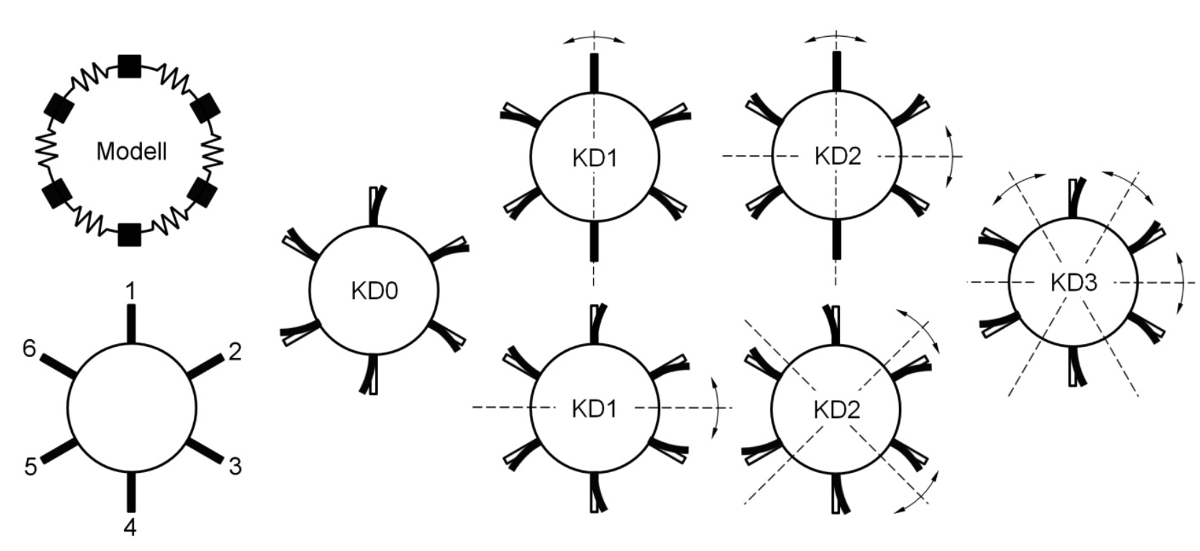
Schwitzke (2015) uses a simplified spring-mass system with \(N\) springs and \(N\) masses, see Figure 10.2 top left. Using this cyclically symmetric structure with six blades, he illustrates the eigenvalue pairs resulting from the solution of the equation of motion \(M\ddot{q} + Kq = 0\) and the associated six natural frequencies and mode shapes.
10.1 Mathematical Derivation
The mathematical considerations in this section follow Strehlau (2011) and Schwitzke (2015). Further information can be found in Zurmühl and Falk (1992) (p. 296, “Zweites Beispiel” (second example), and p. 359, Equations 57 and 59).
The general homogeneous equation of motion \[ M\ddot{q} + (D+G) \dot{q} + Kq = 0 \] with mass matrix \(M\), damping matrix \(D\), stiffness matrix \(K\), the matrix \(G\) of the gyroscopic forces, and the displacement vector \(q\) simplifies for \(D = G = 0\) (undamped, without gyroscopic forces) to \[ M\ddot{q} + Kq = 0. \tag{10.1}\]
Definition 10.1 (Cyclic Oscillator Chain) A cyclic oscillator chain consists of \(N\) identical masses \(m\) connected by \(N\) identical springs with spring constant \(c\) to form a closed ring. Element \(j\) obeys the equation of motion \[ m \ddot{q}_j = -c(q_j - q_{j-1}) - c(q_j - q_{j+1}), \qquad j = 1, \ldots, N, \] with cyclically read indices (\(q_0 := q_N\), \(q_{N+1} := q_1\)). In matrix form, this is Equation 10.1 with the mass matrix \(M = mE\) and the stiffness matrix \[ K = c\,C_N = c \begin{pmatrix} 2 & -1 & 0 & \ldots & 0 & -1 \\ -1 & 2 & -1 & \ldots & 0 & 0 \\ 0 & -1 & 2 & \ldots & 0 & 0 \\ \vdots & \vdots & \vdots & \ddots & \vdots & \vdots \\ 0 & 0 & 0 & \ldots & 2 & -1 \\ -1 & 0 & 0 & \ldots & -1 & 2 \\ \end{pmatrix}, \tag{10.2}\] that is, \(K_{j,j} = 2c\) and \(K_{j,j-1} = K_{j,j+1} = -c\) (cyclically, i.e., \(K_{1,N} = K_{N,1} = -c\)).
The \(j\)-th row of \(K\) thus contains the coefficients of the equation of motion of element \(j\). Both \(M\) and \(K\) are symmetric, and the vector \(q\) has \(N\) degrees of freedom. With the ansatz for a harmonic oscillation \[ q(t) = \hat{q}\, \mathrm{e}^{\lambda t} \] division by \(\mathrm{e}^{\lambda t} \neq 0\) yields the eigenvalue problem \[ \lambda^2 M \hat{q}\, \mathrm{e}^{\lambda t} + K \hat{q}\, \mathrm{e}^{\lambda t} = 0 \quad\Leftrightarrow\quad (\lambda^2 M + K)\hat{q} = 0. \]
Proposition 10.1 (Natural Angular Frequencies of the Cyclic Oscillator Chain) The eigenvalue problem \((\lambda^2 M + K)\hat{q} = 0\) of the cyclic oscillator chain has \(N\) solutions for \(\lambda^2\) and thus \(2N\) eigenvalues \(\lambda_{k\pm} = \pm\mathrm{j}\omega_k\) with the natural angular frequencies \[ \omega_k = 2\sqrt{\frac{c}{m}}\,\left|\sin\frac{\pi k}{N}\right|, \qquad k = 0, 1, \ldots, N-1. \]
Proof. Since \(M = mE\) and \(K = c\,C_N\), we have \(\lambda^2 = -\frac{c}{m}\mu_k\), where \(\mu_k\) are the eigenvalues of \(C_N\). By Theorem 8.16 and its subsequent generalization to all eigenvectors of \(C_n\), \(\mu_k = 2 - 2\cos(2\pi k/N) = 4\sin^2(\pi k/N)\), \(k = 0, \ldots, N-1\). Hence \(\lambda = \pm\mathrm{j}\,2\sqrt{c/m}\,\lvert\sin(\pi k/N)\rvert\).
For \(k = 0\) the natural angular frequency vanishes: the ring moves as a whole without stretching any spring. The eigenvalue \(\lambda = 0\) is then double, and the associated component of the solution is \((A_0 + B_0 t)\,\hat{q}_0\) instead of an oscillation.
The solution is the superposition of the \(N\) partial solutions with the eigenvectors \(\hat{q}_k\), \[ q(t) = (A_0 + B_0 t)\,\hat{q}_0 + \sum_{k=1}^{N-1} \hat{q}_k \left( \underline{C}_k\, \mathrm{e}^{-\mathrm{j} \omega_k t} + \overline{\underline{C}}_k\, \mathrm{e}^{+\mathrm{j} \omega_k t} \right) \tag{10.3}\] with constant, mutually complex conjugate coefficients \(\underline{C}_k = \tfrac{1}{2}(A_k + \mathrm{j}B_k)\) and \(\overline{\underline{C}}_k = \tfrac{1}{2}(A_k - \mathrm{j}B_k)\). Euler’s formula then yields the real solution \[ q(t) = (A_0 + B_0 t)\,\hat{q}_0 + \sum_{k=1}^{N-1} \left( A_k \cos(\omega_k t) + B_k \sin(\omega_k t) \right) \hat{q}_k. \tag{10.4}\]
The eigenvalues \(\lambda_{k\pm}\) follow from the natural angular frequencies \(\omega_k\); the eigenvectors \(\hat{q}_k\) are the associated mode shapes.
Proposition 10.2 (Mode Shapes of the Cyclic Oscillator Chain) For \(0 < k < N/2\), the indices \(k\) and \(N-k\) share the same natural angular frequency \(\omega_k = \omega_{N-k}\). The associated eigenvectors \[ \hat{q}_{k} = \begin{pmatrix} \cos(1 \times 2 \pi k /N) \\ \cos(2 \times 2 \pi k /N) \\ \vdots \\ \cos(j \times 2 \pi k /N) \\ \vdots \\ \cos(N \times 2 \pi k /N) \\ \end{pmatrix} \tag{10.5}\] and \[ \hat{q}_{N-k} = \begin{pmatrix} \sin(1 \times 2 \pi k /N) \\ \sin(2 \times 2 \pi k /N) \\ \vdots \\ \sin(j \times 2 \pi k /N) \\ \vdots \\ \sin(N \times 2 \pi k /N) \\ \end{pmatrix} \tag{10.6}\] are mutually orthogonal. The \(j\)-th row contains the displacement of the \(j\)-th element of the oscillator chain. For \(k = 0\) and, for even \(N\), for \(k = N/2\), only the cosine vector Equation 10.5 is an eigenvector.
Proof. As shown after Theorem 8.16, \((\zeta^{k}, \zeta^{2k}, \ldots, \zeta^{Nk})^T\) with \(\zeta = \mathrm{e}^{2\pi\mathrm{j}/N}\) is an eigenvector of \(C_N\) for the real eigenvalue \(\mu_k\). Since \(C_N\) is real, the real and imaginary parts of this vector are also eigenvectors for \(\mu_k\). These are Equation 10.5 and Equation 10.6. For \(k = 0\) and \(k = N/2\) the imaginary part vanishes. Orthogonality follows from \(\sum_{j=1}^{N} \cos(2\pi jk/N)\sin(2\pi jk/N) = \tfrac12 \sum_{j=1}^{N} \sin(4\pi jk/N) = 0\) for \(2k \neq N\).
10.2 Interpretation of the Mathematical Considerations
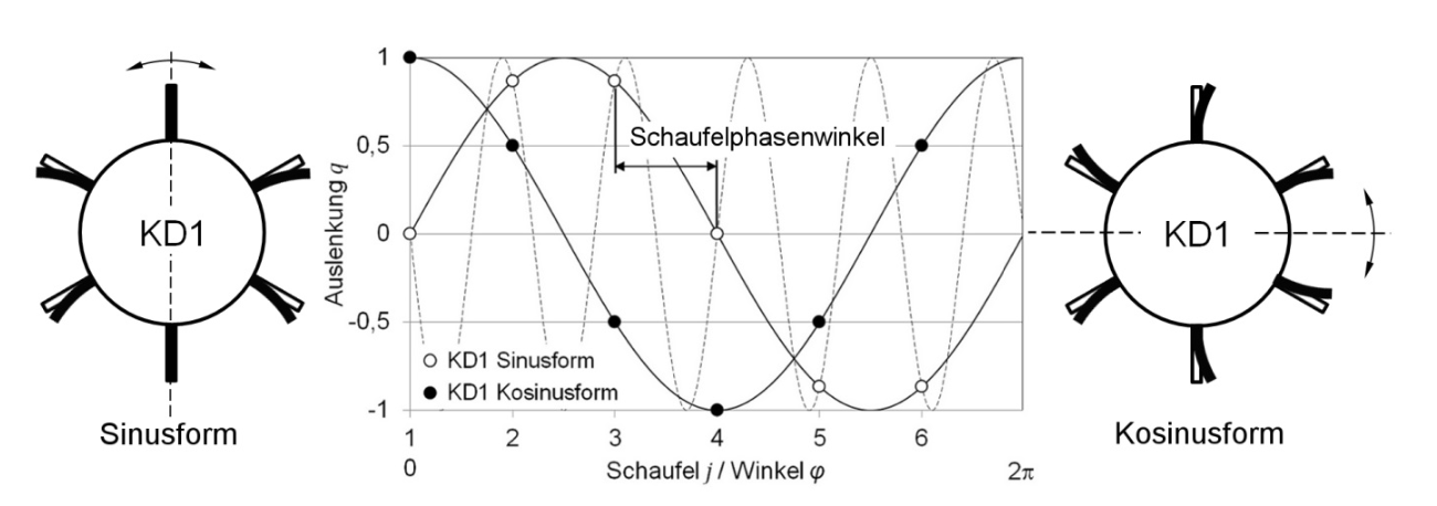
Section 10.1 yields the following relationships. For \(k = 0\), the eigenvector shows that all blades are maximally displaced at the same time. This corresponds to the KD0 mode shape in Figure 10.2 (bottom left), for which a single eigenvalue occurs. The indices \(k\) and \(N-k\) yield a cosine- or sine-shaped deformation along the circumference, that is, a mode shape with \(k = \mathrm{KD}\) nodal diameters, see Figure 10.3.
For an even number \(N\) of blade-disk sectors, \(k = N/2\) also has only a single solution; in the case considered (Figure 10.2), this is the KD3 mode shape. All remaining eigenvalues, i.e., for odd \(N\) all those with \(k \neq 0\), occur twice. Their two eigenvectors are mutually orthogonal, which, as in Figure 10.3, shows up as a position of the nodal diameter lines rotated by the angle \(\pi/(2\,\mathrm{KD})\).
At the maximum number of nodal diameters, all adjacent blades vibrate in antiphase. For odd numbers of blades, one blade does not participate in the vibration at \(\mathrm{KD}_{\max}\) if the nodal diameter line passes through it. Mode shapes with \(\mathrm{KD} > \mathrm{KD}_{\max}\) are confined to the disk, since the cyclically symmetric structure, with its limited number of blade-disk sectors, cannot represent such vibrations. For example, the dashed KD5 mode shape in Figure 10.3 exhibits the same blade displacements as the one with a single nodal diameter. The maximum number of nodal diameters follows from the number \(N\) of blades: \[ \mathrm{KD}_{\max} = \begin{cases} N/2 & \text{for even } N,\\ (N-1)/2 & \text{for odd } N. \end{cases} \tag{10.7}\]
10.3 Phase Angle of the Blades
According to Equation 10.3 or Equation 10.4, the \(j\)-th blade, i.e., the \(j\)-th element of the oscillator chain, performs a harmonic oscillation that can be represented either in complex exponential form or with trigonometric functions. A single mode shape describes an in-phase vibration of all blades with nodal diameter lines fixed relative to the structure. Since the double eigenvalue pairs share the same natural frequency, both mode shapes occur superimposed under excitation. Their superposition yields a rotating mode shape. Since the nodal diameter lines have no preferred direction in the ideal system, they rotate counterclockwise or clockwise, as indicated in Figure 10.2. The blades perform a wave motion and consequently do not vibrate in phase.
Definition 10.2 (Inter-Blade Phase Angle) The inter-blade phase angle (blade phase angle) is the phase difference between two adjacent blades of a rotating mode shape with \(\mathrm{KD}\) nodal diameters, \[ \varphi_{\mathrm{KD}} = \frac{2 \pi\, \mathrm{KD}}{N}. \]
Figure 10.3 shows the inter-blade phase angle for KD1. Each blade experiences its maximum displacement at a different time and leads or lags the adjacent blade by \(\varphi_{\mathrm{KD}}\).
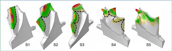
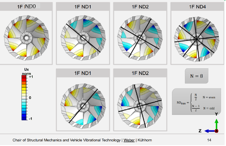
ND0 to ND4) of the disk for the first blade vibration mode S1 from Figure 10.4. The deformation of the blades along the circumference is shown as a function of the nodal diameter of the disk; ND0 to ND4 correspond to KD0 to KD4. Source: MAN Energy Solution SE (2023)