import numpy as np
from scipy.linalg import toeplitz
K4 = toeplitz([2, -1, 0, 0])
print(K4)
[[ 2 -1 0 0]
[-1 2 -1 0]
[ 0 -1 2 -1]
[ 0 0 -1 2]]This chapter is based on Strang (2010). It treats four special families of matrices: \(K_n\), \(C_n\), \(T_n\), and \(B_n\). The family \(C_n\) in particular is important for the solution of Exercise 11.1. The symbols of this chapter are listed in Table 8.1.
| Symbol | Meaning | Type | Defined in |
|---|---|---|---|
| \(a\) | Constant coefficient of a linear ODE (\(y' + ay = g(x)\); growth rate in \(y' = ay\)) | Constant | Section 8.5.2 |
| \(c\) | Spring constant | Constant | Theorem 2.7 |
| \(c_i\) | Spring constant of spring \(i\) (\(c_{12}\): coupling spring) | Constant | Section 8.6 |
| \(\mathrm{d}\) | Differential (\(\mathrm{d}x\), \(\frac{\mathrm{d}y}{\mathrm{d}x}\)) | Operator | Example 2.1 |
| \(\mathrm{e}\) | Euler’s number | Constant | Example 2.1 |
| \(e, e_i\) | Elongation (strain) of spring \(i\); vector \(e = Au\) | Vector | Section 8.6 |
| \(f, f_j\) | Vector of external forces (right-hand side of \(Ku = f\)); \(f_j\) force on mass \(j\), \(f_0\) reaction force at the upper end | Vector | Section 8.1 |
| \(g\) | Gravitational acceleration | Constant | Equation 2.28 |
| \(h\) | Step size of an integration scheme; grid spacing \(h = 1/(n+1)\) | Scalar | Definition 3.1, Section 8.5.5 |
| \(i\) | Running index (component, row, eigenvalue number, spring number) | Index | Section 8.1 |
| \(j\) | Running index (row/column, mass, blade); typographically distinct from \(\mathrm{j}\) | Index | Section 8.1 |
| \(\mathrm{j}\) | Imaginary unit, \(\mathrm{j}^2 = -1\) | Constant | Theorem 2.4 |
| \(k\) | Running index (time/iteration step, mode, eigenvalue number) | Index | Definition 3.1 |
| \(l_0\) | Rest length of a spring | Constant | Figure 8.5 |
| \(\ell\) | Running index (component of an eigenvector, solution number) | Index | Section 8.5.5 |
| \(m\) | Mass | Constant | Theorem 2.6 |
| \(m_i\) | Mass \(i\) | Constant | Section 8.6 |
| \(n\) | Order of an ODE; dimension of a matrix or system; number of steps | Index | Section 8.1 |
| \(r\) | Number of springs (rows of the difference matrix \(A\)) | Index | Section 8.6 |
| \(t\) | Time | Scalar | Section 8.5.2 |
| \(u, u_i\) | Displacement vector of the masses (unknown in \(Ku = f\)); \(u_i\) displacement of mass \(i\) | Vector | Section 8.1 |
| \(v, v_i\) | Eigenvector; \(v_i\) eigenvector for the eigenvalue \(\lambda_i\) or \(\mu_k\) | Vector | Definition 5.1 |
| \(w, w_i\) | Internal spring force (tension) of spring \(i\), vector \(w = Ce\) | Vector | Section 8.6 |
| \(x\) | Independent variable (Ch. 02 §1–4, 03, 06, 08 eigenfunctions) | Scalar | Theorem 8.11 |
| \(y\) | Unknown function \(y(x)\) or vector of unknown functions; \(y', y'', y^{(n)}\) derivatives | Function | Section 8.5.2 |
| \(y_k(x)\) | Eigenfunction of \(-y'' = \lambda y\) for the boundary condition | Function | Theorem 8.11 |
| \(z\) | Complex number | Scalar | Figure 8.2 |
| \(A\) | Matrix (coefficient, system, or difference matrix, \(e = Au\)) | Matrix | Definition 5.1 |
| \(A, B\), \(A_i, B_i\) | Coefficients of the real modal solution, \(q(t) = \sum (A_k\cos\omega_k t + B_k \sin\omega_k t)\hat{q}_k\) (\(A_i, B_i\) in 08) | Scalar | Theorem 8.19, Equation 8.3 |
| \(B\) | Further matrix (similar matrix \(A = P^{-1}BP\); \(B = A - \lambda E\) in the brute-force (“Hau-Ruck”) method) | Matrix | Definition 5.2 |
| \(B_n\) | Family of matrices with free ends: tridiagonal \(-1, 2, -1\), first and last diagonal entry \(1\) | Matrix | Section 8.3 |
| \(C\) | Constant of integration; \(C_1, \dots, C_n\) constants of integration or coefficients of the general solution | Constant | Example 2.1 |
| \(C\) | Diagonal matrix of the spring constants \(c_i\) in \(K = A^TCA\) | Matrix | Section 8.6 |
| \(C_n\) | Circulant matrix (\(-1, 2, -1\) cyclic); \(C_N\) for the ring of \(N\) masses | Matrix | Definition 8.2 |
| \(D\) | Diagonal matrix of the pivots in \(LDL^T\) (only in the name of the factorization) | Matrix | Theorem 8.1 |
| \(E\) | Identity matrix | Matrix | Definition 5.1 |
| \(F\) | Force; \(F(t)\) external force, \(F_0\) its amplitude, \(F_1, F_2, F_3\) component forces, \(F_{\mathrm{R}}\) restoring force, \(F_{\mathrm{G}}\) weight | Scalar | Theorem 2.6 |
| \(H_3\) | “Hanging matrix” (fixed-free, \(3 \times 3\)) | Matrix | Section 8.6 |
| \(J\) | Jordan matrix | Matrix | Table 8.2 |
| \(K\) | Stiffness matrix, \(K = A^TCA\) | Matrix | Definition 8.5 |
| \(K_n\) | Family of second difference matrices: tridiagonal \(-1, 2, -1\) (fixed-fixed) | Matrix | Section 8.1 |
| \(K_{ij}\) | Element of the matrix \(K\) in row \(i\), column \(j\) | Scalar | Section 8.1 |
| \(L\) | Lower triangular matrix in \(LDL^T\) or \(LL^T\) (Cholesky) | Matrix | Theorem 8.1 |
| \(M\) | Mass matrix, \(M = \operatorname{diag}(m_1, \dots, m_n)\) | Matrix | Definition 8.5 |
| \(P\) | Invertible matrix of a similarity transformation, \(A = P^{-1}BP\) | Matrix | Definition 5.2 |
| \(Q\) | Orthogonal matrix, \(Q^T Q = E\); columns are orthonormal eigenvectors | Matrix | Theorem 8.10 |
| \(T_n\) | Fixed-free family of matrices: tridiagonal \(-1, 2, -1\), first diagonal entry \(1\) | Matrix | Section 8.2 |
| \(U\) | Upper triangular matrix from elimination | Matrix | Section 8.2 |
| \(U, \Sigma, V\) | Factors of the singular value decomposition \(A = U\Sigma V^T\) (only in Table 8.2) | Matrix | Table 8.2 |
| \(V\) | Eigenvector matrix (columns \(v_1, \dots, v_n\)), \(V^{-1}AV = \Lambda\) | Matrix | Theorem 8.6 |
| \(\mathbb{R}\), \(\mathbb{R}^n\) | Set of real numbers or of \(n\)-tuples | Set | Figure 8.4 |
| \(\alpha\) | Rigid-body displacement: all masses by the same amount, \(u = (\alpha, \dots, \alpha)\) | Scalar | Section 8.1 |
| \(\gamma_i\) | Coefficient of a linear combination (weights of the RK2 method; expansion of the starting vector in eigenvectors; basis representation in the eigenspace) | Scalar | Example 8.2 |
| \(\Delta t, \Delta x\) | Time step; spatial grid spacing | Scalar | Section 8.7, Section 8.5.5 |
| \(\theta\) | Angle: \(\theta = k\pi/(n+1)\) or \(2\pi k/n\) (discrete sine/exponential function) | Scalar | Section 8.5.5 |
| \(\lambda\) | Eigenvalue or root of the characteristic equation (exponent in the ansatz \(\mathrm{e}^{\lambda t}\)); \(\lambda_i\), \(\lambda_k\) | Scalar | Definition 5.1 |
| \(\Lambda\) | Diagonal matrix of the eigenvalues | Matrix | Theorem 8.6 |
| \(\pi\) | The number pi (italic, KaTeX exception) | Constant | – |
| \(\omega\) | Angular frequency (excitation angular frequency; imaginary part of an eigenvalue; frequency of an eigenfunction) | Scalar | Theorem 8.11 |
| \(\omega_0\) | Natural angular frequency of the undamped single-mass oscillator, \(\omega_0 = \sqrt{c/m}\) (simple pendulum: \(\sqrt{g/l}\)) | Constant | Equation 2.8 |
| \(\zeta\) | \(n\)-th root of unity, \(\zeta = \mathrm{e}^{2\pi\mathrm{j}/n}\); \(\overline{\zeta}\) conjugate | Scalar | Theorem 8.15 |
| \(y', y'', y^{(n)}\) | First, second, \(n\)-th derivative with respect to the independent variable | Operator | Example 2.1 |
| \(\dot{x}, \ddot{x}\) | First and second derivative with respect to time \(t\) | Operator | Equation 2.8 |
| \(\sum\) | Sum | Operator | Equation 8.3 |
| \(A^T\) | Transpose | Operator | Section 8.1 |
| \(A^{-1}\) | Inverse | Operator | Section 8.1 |
| \(\det\) | Determinant | Operator | Theorem 8.5 |
| \(\operatorname{Re}, \operatorname{Im}\) | Real and imaginary parts | Operator | Table 8.2 |
| \(\operatorname{diag}\) | Diagonal matrix formed from entries | Operator | Section 8.7 |
| \(\mathrm{DST}\) | Matrix of the discrete sine transform | Matrix | Definition 8.6 |
| \(\overline{\lambda}\) | Complex conjugate | Operator | Theorem 8.16 |
| \(\lVert v \rVert\), \(\lvert z \rvert\) | Euclidean norm, absolute value | Operator | Section 8.5.6 |
| local | \(A, B\) (example matrices in Example 8.1 and Section 8.5.6.1), \(y_\ell\) (samples \(\sin(\ell\theta)\), \(\cos(\ell\theta)\) in Section 8.5.5), \(u, v\) (arbitrary vectors in the rows “reflection” and “rank 1” of Table 8.2) | local | where used |
This section refers to Chapter 1.1 in Strang (2010).
An \(r \times n\) matrix has \(r\) rows, \(n\) columns, and \(rn\) entries. We operate on these rows and columns to solve systems of linear equations \(Au = f\) and eigenvalue problems \(Av = \lambda v\). From the inputs \(A\) and \(f\) we obtain (with the help of software such as Python) the outputs \(u\), or \(\lambda\) and \(v\). A fast and stable algorithm is extremely important here.
Matrices are used to store information. In applied mathematics, however, we often regard them as an “operator”: the matrix \(A\) acts on vectors \(u\) and produces other vectors \(Au\). The components of \(u\) have a meaning: they stand for displacements, pressures, voltages, prices, or concentrations. The operator \(A\) also has a meaning: it forms differences. So the components of \(Au\) are pressure differences, voltage drops, or price differences.
We consider four special families of matrices. They are simple, useful, and truly fundamental. We first look at the properties of these special matrices \(K_n\), \(C_n\), \(T_n\), and \(B_n\). Some properties are obvious, others are hidden. It is a pleasure to do linear algebra with matrices that really matter.
We begin by describing the matrices \(K_2\), \(K_3\), \(K_4\) from the first family, whose diagonals carry the entries \(-1\), \(2\), and \(-1\):
\[ K_2 = \begin{pmatrix} 2 & -1 \\ -1 & 2 \end{pmatrix}, \]
\[ K_3 = \begin{pmatrix} 2 & -1 & 0 \\ -1 & 2 & -1 \\ 0 & -1 & 2 \end{pmatrix}, \]
\[ K_4 = \begin{pmatrix} 2 & -1 & 0 & 0 \\ -1 & 2 & -1 & 0 \\ 0 & -1 & 2 & -1 \\ 0 & 0 & -1 & 2 \end{pmatrix}. \]
What characterizes the matrices \(K_2\), \(K_3\), \(K_4\), and finally the \(n \times n\) matrix \(K_n\)?
Because \(K\) is a tridiagonal matrix, \(Ku = f\) can be solved quickly. If the unknown vector \(u\) has a thousand components, we can determine them in a few thousand steps (which takes a small fraction of a second on a computer). For a full matrix of order \(n = 1000\), solving \(Ku = f\) would take hundreds of millions of steps. Of course, we must first ask whether the linear equations have a solution at all. We come to this question shortly.
The whole world of Fourier transforms is tied to matrices with constant diagonals. In signal processing, the matrix \(K/4\) serves as a “high-pass filter”. The product \((K/4)u\) selects the rapidly varying (high-frequency) component of a vector \(u\). It is a convolution with \(\frac{1}{4}(-1, 2, -1)\).
Mathematicians call the matrix \(K\) a Toeplitz matrix, and Python uses this name as well: the command K4 = toeplitz([2, -1, 0, 0]) constructs \(K_4\) from row 1.
import numpy as np
from scipy.linalg import toeplitz
K4 = toeplitz([2, -1, 0, 0])
print(K4)[[ 2 -1 0 0]
[-1 2 -1 0]
[ 0 -1 2 -1]
[ 0 0 -1 2]]Definition 8.1 (Toeplitz Matrices) A Toeplitz matrix is a matrix in which all diagonals running from top left to bottom right have the same value. For example, the following matrix is a Toeplitz matrix: \[ \begin{pmatrix} 1 & 2 & 3 & 4 \\ 5 & 1 & 2 & 3 \\ 9 & 5 & 1 & 2 \\ 7 & 9 & 5 & 1 \end{pmatrix}. \]
If we make two small changes in \(K_n\), we obtain the family of matrices \(C_n\): we enter the element \(-1\) in the top right and bottom left corners. This completes two (circulating) diagonals. Each row vector of \(C_4\) is now shifted one entry to the right relative to the row vector above it.
Definition 8.2 (Circulant Matrix) A circulant matrix (also “periodic matrix” or “cyclic convolution”) is a Toeplitz matrix whose diagonals wrap around cyclically: each row arises from the row above it by a shift of one entry to the right, and the entry pushed out at the right edge re-enters at the left edge. The matrices \(C_n\) are circulant. For \(n = 4\), \[ C_4 = \begin{pmatrix} 2 & -1 & 0 & -1 \\ -1 & 2 & -1 & 0 \\ 0 & -1 & 2 & -1 \\ -1 & 0 & -1 & 2 \end{pmatrix}. \]
import numpy as np
from scipy.linalg import toeplitz
C4 = toeplitz([2, -1, 0, -1])
print(C4)[[ 2 -1 0 -1]
[-1 2 -1 0]
[ 0 -1 2 -1]
[-1 0 -1 2]]The matrix \(C_4\) is singular. It is not invertible. Its determinant is zero. Instead of computing this determinant, it is better to find a nonzero vector \(u\) that solves \(C_4u = 0\). (If \(C_4\) had an inverse, the only solution to \(C_4u = 0\) would be the zero vector. We could multiply by \(C_4^{-1}\) to find that \(u = 0\).) For this matrix, it is the column vector of all ones (that is, \(u = (1, 1, 1, 1)\)) that solves the equation \(C_4u = 0\).
The sum of the columns of the matrix \(C_4\) is the zero column. The vector \(u = \begin{pmatrix} 1, & 1, & 1, & 1 \end{pmatrix}^T\) lies in the nullspace of \(C_4\). The nullspace contains all solutions to \(C_4u = 0\).
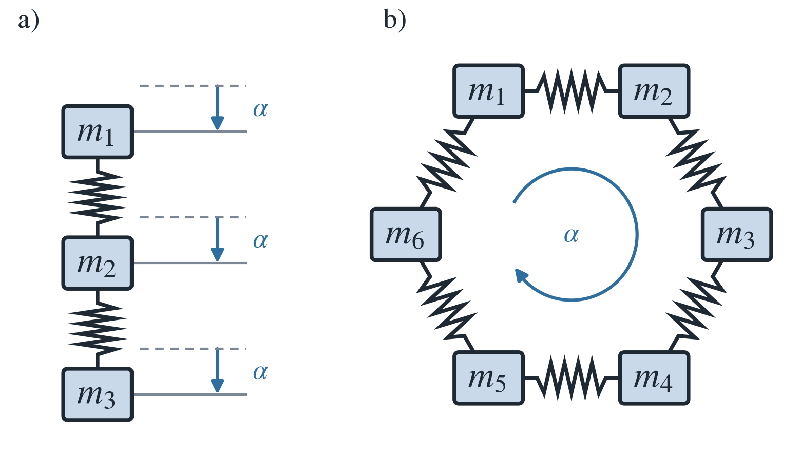
If the entries in every row of a matrix sum to zero, the matrix is certainly singular. The reason is again the column vector of all ones. In the matrix multiplication \(C_4u\), all column vectors are added. Each sum is zero. The constant vector \(u = (1,1,1,1)\), or \(u = (\alpha,\alpha,\alpha,\alpha)\), from the nullspace behaves like the constant \(C\) when integrating a function. In calculus, the “constant of integration” cannot be determined from the derivative. In algebra, the constant \(\alpha\) in \(u = (\alpha,\alpha,\alpha,\alpha)\) cannot be determined from the equation \(C_4u = 0\).
The invertibility of a matrix is not easy to see at a glance. In theory, one could compute the determinant. Only if \(\det K = 0\) does no inverse exist, because computing \(K^{-1}\) involves a division by \(\det K\). In practice, however, the determinant is almost never computed. It is a cumbersome way to determine \(u = K^{-1}f\).
Instead, we proceed with the elimination steps that solve \(Ku = f\). These steps simplify the matrix so that it becomes triangular. This gives us the pivots of the matrix.
Definition 8.3 (Pivots) A pivot is the entry of a matrix that is used during an elimination step to simplify the system of equations. It is typically the first nonzero entry in the current row and lies on the main diagonal. Three operations are allowed to transform the matrix into an upper triangular matrix: adding a multiple of one row to another, multiplying a row by a nonzero scalar, and interchanging two rows. These operations use the pivots by making all entries below the pivots zero. The pivots are therefore the diagonal entries of the resulting upper triangular matrix.
The nonzero pivots on the main diagonal of the triangular matrix show that the original matrix \(K\) is invertible. (Important note: we do not want and do not need \(K^{-1}\) to determine \(u = K^{-1}f\). The inverse would be a full matrix with positive entries. We compute only the solution vector \(u\).)
Definition 8.4 (Positive Definiteness) A symmetric \(n \times n\) matrix \(A\) is called positive definite if \(u^TAu > 0\) holds for all vectors \(u \neq 0\). It is called positive semidefinite if \(u^TAu \geq 0\) holds for all vectors \(u\).
Theorem 8.1 (Pivots) An invertible matrix has \(n\) nonzero pivots. A positive definite symmetric matrix has \(n\) positive pivots.
Proof. We sketch the argument for both parts. A matrix is invertible if and only if elimination transforms it into an upper triangular matrix without a zero row, that is, if and only if all \(n\) pivots are nonzero. A zero row would mean that the system of equations has no unique solution. For a symmetric matrix \(A\), elimination without row exchanges yields the factorization \(A = LDL^T\) with a lower triangular matrix \(L\) whose diagonal entries are \(1\) and the diagonal matrix \(D\) of the pivots. Then \(u^TAu = (L^Tu)^TD(L^Tu)\), and because \(L^T\) is invertible, \(L^Tu\) runs through all nonzero vectors as \(u\) does. Hence \(A\) is positive definite if and only if all pivots in \(D\) are positive.
Example 8.1 (Pivots and Elementary Row Operations) The matrix \[ A = \begin{pmatrix} 1 & 0 & 0 \\ 0 & 2 & 0 \\ 0 & 0 & 3 \end{pmatrix} \] has the pivots \(1\), \(2\), and \(3\) on the main diagonal, all of which are greater than zero. The matrix is positive definite and invertible. If we multiply the last row by \(-1\) (an elementary row operation), we obtain the matrix \[ B = \begin{pmatrix} 1 & 0 & 0 \\ 0 & 2 & 0 \\ 0 & 0 & -3 \end{pmatrix}. \] The pivots of the first two rows are still \(1\) and \(2\), but the pivot of the last row is \(-3\). The matrix \(B\) is not positive definite, but it is invertible, since all pivots are nonzero.
Theorem 8.2 (Eigenvalues) An invertible matrix has \(n\) nonzero eigenvalues. A positive definite symmetric matrix has \(n\) positive eigenvalues.
Positive definiteness can be tested by means of the pivots and eigenvalues. The matrix \(C_4\) is not positive definite because it is singular. In fact, the matrix \(C_4\) has three positive pivots and eigenvalues, so it “almost” passes the test. But its fourth eigenvalue is zero (the matrix is singular). Since none of the eigenvalues is negative (\(\lambda \geq 0\)), \(C_4\) is positive semidefinite (Definition 8.4).
When we solve \(Ku = f\) by elimination, the pivots appear on the main diagonal. The eigenvalues appear in \(Kv = \lambda v\). Positive definiteness can also be tested by means of the determinant (but not simply by \(\det K > 0\)).
Besides the two families \(K_n\) and \(C_n\), there are two further families you need to know. Matrices from these families are symmetric and tridiagonal, like those from the family \(K_n\). For matrices from the family \(T_n\), however, the entry in position \((1,1)\) is not \(2\) but \(1\):
\[ T_1 = \begin{pmatrix} 1 \end{pmatrix}, \]
\[ T_2 = \begin{pmatrix} 1 & -1 \\ -1 & 2 \end{pmatrix}, \]
\[ T_3 = \begin{pmatrix} 1 & -1 & 0 \\ -1 & 2 & -1 \\ 0 & -1 & 2 \end{pmatrix}, \]
\[ T_4 = \begin{pmatrix} 1 & -1 & 0 & 0 \\ -1 & 2 & -1 & 0 \\ 0 & -1 & 2 & -1 \\ 0 & 0 & -1 & 2 \end{pmatrix}. \]
This first row (T stands for “top”) has to do with a new boundary condition whose meaning we will soon understand. For now, we use the matrix \(T_3\) as a perfect demonstration example for elimination. Row operations make the entries below the main diagonal zero.
In two elimination steps we turn the matrix \(T_3\) into the upper triangular matrix \(U\). In the first step we add row 1 to row 2 so that all entries below the first pivot are zero. In the second step we add the new row 2 to row 3 to obtain \(U\):
\[ T_3= \begin{pmatrix} 1 & -1 & 0 \\ -1 & 2 & -1 \\ 0 & -1 & 2 \end{pmatrix} \quad \rightarrow \quad \begin{pmatrix} 1 & -1 & 0 \\ 0 & 1 & -1 \\ 0 & -1 & 2 \end{pmatrix} \quad \rightarrow \quad \begin{pmatrix} 1 & -1 & 0 \\ 0 & 1 & -1 \\ 0 & 0 & 1 \end{pmatrix} = U. \]
All pivots of the matrix \(T_3\) are \(1\). We can apply our test for invertibility (all pivots must be nonzero). The matrix \(T_3\) even passes the test for positive definiteness (three positive pivots). In fact, every matrix \(T_n\) of this family is positive definite, because all pivots are always \(1\).
The matrix \(U\) has an inverse (which is automatically an upper triangular matrix). What is remarkable about this particular inverse \(U^{-1}\) is that all entries above the main diagonal are \(1\):
\[ U_3^{-1} = \begin{pmatrix} 1 & -1 & 0 \\ 0 & 1 & -1 \\ 0 & 0 & 1 \end{pmatrix}^{-1} = \begin{pmatrix} 1 & 1 & 1 \\ 0 & 1 & 1 \\ 0 & 0 & 1 \end{pmatrix}. \]
From this we learn that the inverse of a \(3 \times 3\) “difference matrix” is a \(3 \times 3\) “sum matrix”. The product \(U^{-1}U\) is the identity matrix \(E\). The matrix \(U\) forms differences, its inverse \(U^{-1}\) forms sums. Taking differences first and then sums returns the original vector \((u_1,u_2,u_3)\).
\(U\) produces differences, that is, \[ \begin{pmatrix} 1 & -1 & 0 \\ 0 & 1 & -1 \\ 0 & 0 & 1 \end{pmatrix} \begin{pmatrix} u_1 \\ u_2 \\ u_3 \end{pmatrix} = \begin{pmatrix} u_1 - u_2 \\ u_2 - u_3 \\ u_3 - 0 \end{pmatrix}, \] and \(U^{-1}\) produces sums, that is, \[ \begin{pmatrix} 1 & 1 & 1 \\ 0 & 1 & 1 \\ 0 & 0 & 1 \end{pmatrix} \begin{pmatrix} u_1 - u_2 \\ u_2 - u_3 \\ u_3 - 0 \end{pmatrix} = \begin{pmatrix} u_1 \\ u_2 \\ u_3 \end{pmatrix}. \]
In the fourth family \(B_n\), the last entry is also \(1\) instead of \(2\). The new boundary condition applies to both ends (B stands for “both”). The matrices \(B_n\) are symmetric and tridiagonal. As you will see shortly, they are not invertible. The matrices \(B_n\) are positive semidefinite, but not positive definite:
\[ B_1 = \begin{pmatrix} 0 \end{pmatrix}, \]
\[ B_2 = \begin{pmatrix} 1 & -1 \\ -1 & 1 \end{pmatrix}, \]
\[ B_3 = \begin{pmatrix} 1 & -1 & 0 \\ -1 & 2 & -1 \\ 0 & -1 & 1 \end{pmatrix}. \]
Again, elimination reveals the properties of the matrix. The first \(n - 1\) pivots are \(1\), because nothing has changed here compared with the matrix \(T_n\). But since the last entry of the matrix \(B_3\) is now \(1\), the last entry of the matrix \(U\) changes:
\[ B_3= \begin{pmatrix} 1 & -1 & 0 \\ -1 & 2 & -1 \\ 0 & -1 & 1 \end{pmatrix} \quad \rightarrow \quad \begin{pmatrix} 1 & -1 & 0 \\ 0 & 1 & -1 \\ 0 & -1 & 1 \end{pmatrix} \quad \rightarrow \quad \begin{pmatrix} 1 & -1 & 0 \\ 0 & 1 & -1 \\ 0 & 0 & 0 \end{pmatrix} = U. \]
There are only two pivots. (A pivot must be nonzero.) The last matrix \(U\) is obviously not invertible. Its determinant is zero because the third row contains only zeros. The constant vector \((1,1,1)\) lies in the nullspace of the matrix \(U\) and hence also in the nullspace of the matrix \(B_3\).
The purpose of elimination was to simplify a linear system such as \(B_3u = 0\) without changing its solutions. In this case, we could also have seen that the matrix \(B_3\) is not invertible from the fact that the entries in every row sum to zero. Then the sum of the columns is the zero column. This is exactly what we obtain when we multiply the matrix \(B_3\) by the vector \((1, 1, 1)\).
Let me summarize this section in four points (all matrices considered are symmetric):
eye and onesAs a first step, we want to construct the matrices \(K_n\). For \(n = 3\) we can enter the \(3 \times 3\) matrix row by row in square brackets:
import numpy as np
K3 = np.array([[2, -1, 0], [-1, 2, -1], [0, -1, 2]])
print(K3)[[ 2 -1 0]
[-1 2 -1]
[ 0 -1 2]]For large matrices this approach is too time-consuming. We can also generate the matrix \(K_8\) with the command eye(): the function eye(N, k) generates an identity matrix. The parameter k specifies the position of the diagonal: k=0 denotes the main diagonal, k=1 the first superdiagonal, and k=-1 the first subdiagonal. The matrix \(K_8\) is symmetric.
K8 = 2*np.eye(8) - np.eye(8, k=1) - np.eye(8, k=-1)
print(K8)[[ 2. -1. 0. 0. 0. 0. 0. 0.]
[-1. 2. -1. 0. 0. 0. 0. 0.]
[ 0. -1. 2. -1. 0. 0. 0. 0.]
[ 0. 0. -1. 2. -1. 0. 0. 0.]
[ 0. 0. 0. -1. 2. -1. 0. 0.]
[ 0. 0. 0. 0. -1. 2. -1. 0.]
[ 0. 0. 0. 0. 0. -1. 2. -1.]
[ 0. 0. 0. 0. 0. 0. -1. 2.]]toeplitzThe constant diagonal entries make \(K\) a Toeplitz matrix. The command toeplitz() generates the matrix \(K\) when each diagonal contains only the same entry \(2\), \(-1\), or \(0\).
K8 = toeplitz([2, -1, 0, 0, 0, 0, 0, 0])
print(K8)[[ 2 -1 0 0 0 0 0 0]
[-1 2 -1 0 0 0 0 0]
[ 0 -1 2 -1 0 0 0 0]
[ 0 0 -1 2 -1 0 0 0]
[ 0 0 0 -1 2 -1 0 0]
[ 0 0 0 0 -1 2 -1 0]
[ 0 0 0 0 0 -1 2 -1]
[ 0 0 0 0 0 0 -1 2]]Here we use the command [0]*6 for a zero vector, with which we generate the six zeros in the first row of the matrix \(K_8\):
K8 = toeplitz([2, -1] + [0]*6)
print(K8)[[ 2 -1 0 0 0 0 0 0]
[-1 2 -1 0 0 0 0 0]
[ 0 -1 2 -1 0 0 0 0]
[ 0 0 -1 2 -1 0 0 0]
[ 0 0 0 -1 2 -1 0 0]
[ 0 0 0 0 -1 2 -1 0]
[ 0 0 0 0 0 -1 2 -1]
[ 0 0 0 0 0 0 -1 2]]For an unsymmetric matrix with constant diagonal entries, you need the command toeplitz(col1, row1). With col1 = [1, -1, 0, 0] and row1 = [1, 0, 0], this command generates a \(4 \times 3\) matrix of backward differences that has nonzero entries on only two diagonals, namely the entries \(1\) on one diagonal and the entries \(-1\) on the other.
KTBC(n)To generate the matrices \(T_n\), \(B_n\), and \(C_n\) from the matrix \(K_n\), only individual entries need to be changed. The input is the size \(n\), and four matrices are generated.
The function K, T, B, C = KTBC(n) generates the four special matrices under the assumption \(n > 1\), using the following rules (in MATLAB notation after Strang (2010)):
K = toeplitz([2 -1 zeros(1,n-2)]);T = K; T(1,1) = 1;B = K; B(1,1) = 1; B(n,n) = 1;C = K; C(1,n) = -1; C(n,1) = -1;It can be implemented in Python as follows:
import numpy as np
from scipy.linalg import toeplitz
def KTBC(n):
K = toeplitz([2, -1] + [0]*(n-2))
T = K.copy()
T[0,0] = 1
B = K.copy()
B[0,0] = 1
B[n-1,n-1] = 1
C = K.copy()
C[0,n-1] = -1
C[n-1,0] = -1
return K, T, B, C
n= 4
K, T, B, C = KTBC(n)
print(f"K{n} = \n{K}")
print(f"T{n} = \n{T}")
print(f"B{n} = \n{B}")
print(f"C{n} = \n{C}")K4 =
[[ 2 -1  0  0]
 [-1  2 -1  0]
 [ 0 -1  2 -1]
 [ 0  0 -1  2]]
T4 =
[[ 1 -1 0 0]
[-1 2 -1 0]
[ 0 -1 2 -1]
[ 0 0 -1 2]]
B4 =
[[ 1 -1 0 0]
[-1 2 -1 0]
[ 0 -1 2 -1]
[ 0 0 -1 1]]
C4 =
[[ 2 -1  0 -1]
 [-1  2 -1  0]
 [ 0 -1  2 -1]
[-1 0 -1 2]]Strang (2010) treats further properties of the matrices \(K_n\), \(T_n\), \(B_n\), and \(C_n\): which boundary conditions these finite difference matrices correspond to, how elimination produces pivots in \(D\) and triangular factors in \(LDL^T\), how point loads lead to the inverse matrices \(K^{-1}\) and \(T^{-1}\), and why the eigenvalues and eigenvectors involve sines and cosines. We take up only some of these topics in order to develop solution ideas for Exercise 11.1, and refer to the book for a comprehensive treatment.
This section refers to Chapter 1.5 in Strang (2010).
This section begins with the equation \(Av = \lambda v\) for an eigenvector \(v\) and its eigenvalue \(\lambda\). For small matrices \(A\) we can solve \(Av = \lambda v\) by starting from \(\det(A - \lambda E) = 0\). You may already be familiar with this (for large matrices this method would be dreadful). There is no “elimination” that delivers the exact eigenvalue \(\lambda\) and the exact eigenvector \(v\) in finite time. Since \(\lambda\) is multiplied by \(v\), the equation \(Av = \lambda v\) is not linear.
A major success of numerical linear algebra is the development of fast and stable algorithms for computing eigenvalues (especially for symmetric matrices \(A\)). The Python command eig(A) does not return an equation but \(n\) numbers \(\lambda_1, \ldots, \lambda_n\). In this chapter, however, we deal with special matrices! For these we will therefore determine \(\lambda\) and \(v\) exactly.
Almost every vector changes its direction when multiplied by a matrix \(A\). Certain exceptional vectors \(v\) lie on the same line as \(Av\). These are the eigenvectors. For an eigenvector, \(Av\) is the original vector \(v\) multiplied by a number \(\lambda\).
The eigenvalue \(\lambda\) tells us whether the special vector \(v\) is stretched, shrunk, reversed, or left unchanged when multiplied by the matrix \(A\). Possible cases are, for example, \(\lambda = 2\) (stretching), \(\lambda = \frac{1}{2}\) (shrinking), \(\lambda = -1\) (reversal), or \(\lambda = 1\) (steady state, since \(Av = v\)).
Theorem 8.3 (Eigenvalue Zero) \(\lambda = 0\) can also occur. If the nullspace contains nonzero vectors, then \(Av = 0v\) holds for them. So the nullspace contains eigenvectors belonging to \(\lambda = 0\).
Theorem 8.4 (The Zero Vector) The zero vector is not an eigenvector. It is not changed by multiplication with a matrix. Although \(A0 = \lambda 0\) holds for every \(\lambda\), the zero vector does not count as an eigenvector by definition.
For our special matrices we will guess \(v\) and then determine \(\lambda\). In the general case we determine \(\lambda\) first. To separate \(\lambda\) from \(v\), we first rewrite the basic equation: \[ Av = \lambda v \text{ means } (A-\lambda E)v = 0. \] The matrix \(A-\lambda E\) must be singular. Its determinant must be zero. The eigenvector \(v\) lies in the nullspace of \(A - \lambda E\). First we note that \(\lambda\) is an eigenvalue if and only if the shifted matrix \(A - \lambda E\) is not invertible:
Theorem 8.5 (Eigenvalues: Characteristic Equation) The number \(\lambda\) is an eigenvalue of \(A\) if and only if \(\det(A - \lambda E) = 0\).
This “characteristic equation” \(\det(A - \lambda E) = 0\) involves only the eigenvalue \(\lambda\), not the eigenvector \(v\). The determinant of \(A-\lambda E\) is a polynomial of degree \(n\) in \(\lambda\). By the fundamental theorem of algebra, this polynomial must have \(n\) roots \(\lambda_1, \ldots, \lambda_n\). Some of these eigenvalues may have a higher multiplicity or be complex. In these cases we have a little more work to do.
When we deal with an eigenvector, multiplication by \(A\) reduces to multiplication by a number: \(Av = \lambda v\). All the difficulties with the \(n \times n\) multiplications disappear. Instead of having to treat a coupled system, we can now consider the eigenvectors one at a time. It is as if we had a diagonal matrix in which the couplings through off-diagonal entries are absent.
With the help of the eigenvalues, we can also easily determine the \(100\)th power of a diagonal matrix. The matrix \(A\) turns into a diagonal matrix \(\Lambda\) when we use the eigenvectors correctly. This is the matrix form of our key idea. The only essential computation follows.
Theorem 8.6 (Diagonalization of a Matrix) Suppose the \(n \times n\) matrix \(A\) has \(n\) linearly independent eigenvectors \(v_1, \ldots, v_n\). These are the columns of an eigenvector matrix \(V\). Then the matrix \(V^{-1}AV = \Lambda\) is diagonal: \[ V^{-1}AV = \Lambda = \begin{pmatrix} \lambda_1 & & \\ & \ddots & \\ & & \lambda_n \end{pmatrix} = \text{eigenvalue matrix}. \tag{8.1}\]
With Equation 8.1, \(K_2^{100}\) can easily be determined using the eigenvalues and eigenvectors of the matrix \(K_2\).
Example 8.2 (Eigenvalues and Eigenvectors of the Matrix \(K_2\)) We compute the eigenvalues and eigenvectors of the matrix \(K_2\) numerically in Python.
import numpy as np
from scipy.linalg import eig
K2 = np.array([[2, -1], [-1, 2]])
eigenvalues, eigenvectors = eig(K2)
print(f"Eigenvalues of K2: {eigenvalues}")
print(f"Eigenvectors of K2: {eigenvectors}")
Eigenvalues of K2: [3.+0.j 1.+0.j]
Eigenvectors of K2: [[ 0.70710678 0.70710678]
[-0.70710678 0.70710678]]As expected, the matrices \(K_2 - E\) and \(K_2 - 3E\) are singular. Each nullspace is a line of eigenvectors. We choose \(v_1\) and \(v_2\) so that they have the simple components \(1\) and \(-1\). Arbitrary (nonzero) multiples \(\gamma_1 v_1\) and \(\gamma_2 v_2\) would have been just as good as eigenvectors. Python chooses \(\gamma_1\) and \(\gamma_2\) with absolute value \(\frac{1}{\sqrt{2}}\), because the eigenvectors then have length \(1\) (that is, they are unit vectors).
If we use SymPy, a free Python library for symbolic mathematics, we obtain the exact eigenvalues and eigenvectors:
import sympy as sp
K2 = sp.Matrix([[2, -1], [-1, 2]])
eigenvalues = K2.eigenvals()
eigenvectors = K2.eigenvects()
for i, (eigenvalue, multiplicity, eigenvector) in enumerate(eigenvectors):
    print(f"Eigenvalue {i+1}: {eigenvalue}")
    print(f"Eigenvector {i+1}: {eigenvector}\n")
Eigenvalue 1: 1
Eigenvector 1: [Matrix([
[1],
[1]])]
Eigenvalue 2: 3
Eigenvector 2: [Matrix([
[-1],
[ 1]])]
Thus we obtain the eigenvector \((1, 1)\) for the eigenvalue \(\lambda = 1\) and the eigenvector \((-1, 1)\) for the eigenvalue \(\lambda = 3\), that is, after normalization, \(\frac{1}{\sqrt{2}}(1, 1)\) and (after multiplication by \(-1\)) \(\frac{1}{\sqrt{2}}(1, -1)\). These eigenvectors of the matrix \[ K_2 = \begin{pmatrix} 2 & -1 \\ -1 & 2 \end{pmatrix} \] are special (just like the matrix \(K_2\) itself).
Theorem 8.7 (Orthogonal Eigenvectors of Symmetric Matrices) Every symmetric \(n \times n\) matrix has a complete set of \(n\) orthogonal unit eigenvectors.
A single ODE \(\frac{\mathrm{d}y}{\mathrm{d}t} = ay\) has the general solution \(y(t) = C\mathrm{e}^{at}\). The initial value \(y(0)\) determines the constant \(C\). The solution \(y(t) = y(0)\mathrm{e}^{at}\) decays for \(a < 0\) and grows for \(a > 0\). Decay stands for stability, growth for instability. If \(a\) is a complex number, its real part decides between growth and decay. The imaginary part \(\omega\) provides an oscillation factor \(\mathrm{e}^{\mathrm{j}\omega t} = \cos\omega t + \mathrm{j}\sin\omega t\).
Now we consider two coupled ODEs for the components of the vector \(u = (u_1, u_2)^T\), which together form the vector equation \(\frac{\mathrm{d}u}{\mathrm{d}t} = Au\):
\[\begin{align*} \frac{\mathrm{d}u_1}{\mathrm{d}t} &= 2u_1 - u_2, \\ \frac{\mathrm{d}u_2}{\mathrm{d}t} &= -u_1 + 2u_2, \end{align*}\] or \[\begin{align*} \frac{\mathrm{d}}{\mathrm{d}t} \begin{pmatrix} u_1 \\ u_2 \end{pmatrix} = \begin{pmatrix} 2 & -1 \\ -1 & 2 \end{pmatrix} \begin{pmatrix} u_1 \\ u_2 \end{pmatrix} \end{align*}\] or equivalently \[\begin{align*} \frac{\mathrm{d}}{\mathrm{d}t} \begin{pmatrix} u_1 \\ u_2 \end{pmatrix} = K_2 \begin{pmatrix} u_1 \\ u_2 \end{pmatrix}. \end{align*}\]
The solution will still contain exponential functions \(\mathrm{e}^{\lambda t}\). But there is no longer a single growth rate as in \(\mathrm{e}^{at}\). The associated matrix \(A = K_2\) has two eigenvalues \(\lambda_1 = 1\) and \(\lambda_2 = 3\). The solution therefore contains two exponential functions \(\mathrm{e}^t\) and \(\mathrm{e}^{3t}\). They are multiplied by the eigenvectors \(v_1 = (1, 1)\) and \(v_2 = (1, -1)\).
The correct way to find solutions is via the eigenvectors. The pure solutions \(\mathrm{e}^{\lambda t}v\) are eigenvectors that grow according to their own eigenvalue \(1\) or \(3\). We combine them: \[ u(t) = C_1\mathrm{e}^tv_1 + C_2\mathrm{e}^{3t}v_2 \] gives \[ u_1(t) = C_1\mathrm{e}^t + C_2\mathrm{e}^{3t}, \quad u_2(t) = C_1\mathrm{e}^t - C_2\mathrm{e}^{3t}, \] or in matrix notation \[ \begin{pmatrix} u_1(t) \\ u_2(t) \end{pmatrix} = C_1 \begin{pmatrix} 1 \\ 1 \end{pmatrix} \mathrm{e}^t + C_2 \begin{pmatrix} 1 \\ -1 \end{pmatrix} \mathrm{e}^{3t}. \]
This is the complete solution. The two constants \(C_1\) and \(C_2\) are determined by the two initial values \(u_1(0)\) and \(u_2(0)\). First convince yourself that each pure solution \(\mathrm{e}^{\lambda t}v\) solves the equation \(\frac{\mathrm{d}u}{\mathrm{d}t} = Au\):
Theorem 8.8 (Eigenvectors and Solutions) If \(v\) is an eigenvector of \(A\) for the eigenvalue \(\lambda\), then \(u(t) = \mathrm{e}^{\lambda t}v\) solves the ODE \(\frac{\mathrm{d}u}{\mathrm{d}t} = Au\).
\(\square\)
Proof. We have \(\frac{\mathrm{d}u}{\mathrm{d}t} = \lambda \mathrm{e}^{\lambda t}v = \mathrm{e}^{\lambda t}Av = Au\).
The number \(\mathrm{e}^{\lambda t}\) is just a factor by which all components of the eigenvector \(v\) are multiplied. This is the essential property of eigenvectors: they grow or decay at their own rate \(\lambda\). The complete solution \(u(t)\) is a combination of the pure modes \(C_1\mathrm{e}^tv_1\) and \(C_2\mathrm{e}^{3t}v_2\).
With Theorem 8.6, this computation can be carried out in general in three steps. One decomposes the initial value in terms of the eigenvectors, \(u(0) = C_1v_1 + \cdots + C_nv_n\), multiplies each \(C_i\) by \(\mathrm{e}^{\lambda_i t}\), and obtains \[ u(t) = C_1\mathrm{e}^{\lambda_1 t}v_1 + \cdots + C_n\mathrm{e}^{\lambda_n t}v_n = V\mathrm{e}^{\Lambda t}V^{-1}u(0), \] where \(\mathrm{e}^{\Lambda t}\) is the diagonal matrix with the entries \(\mathrm{e}^{\lambda_i t}\) and the vector \(V^{-1}u(0)\) contains the constants \(C_1, \ldots, C_n\).
Example 8.3 (Initial Values and Eigenvectors of the Matrix \(K_2\)) Suppose the initial values are \(u_1(0) = 7\) and \(u_2(0) = 3\). These determine the constants \(C_1\) and \(C_2\). At the starting time \(t = 0\), both growth factors \(\mathrm{e}^{\lambda t}\) equal one: \[ u(0) = C_1 \begin{pmatrix} 1 \\ 1 \end{pmatrix} + C_2 \begin{pmatrix} 1 \\ -1 \end{pmatrix} \text{ is } \begin{pmatrix} 7 \\ 3 \end{pmatrix} = 5 \begin{pmatrix} 1 \\ 1 \end{pmatrix} + 2 \begin{pmatrix} 1 \\ -1 \end{pmatrix}. \]
We solve the two equations and obtain \(C_1 = 5\) and \(C_2 = 2\). The complete solution is therefore \(u(t) = 5\mathrm{e}^tv_1 + 2\mathrm{e}^{3t}v_2\). It is a combination of a slower and a faster growth. For large \(t\), the faster-growing \(\mathrm{e}^{3t}\) dominates, so the solution points in the direction of \(v_2\).
In Section 8.7 we will discuss the important equation \(M\ddot{u} + Ku = 0\) in more detail.
Newton’s law involves acceleration (the second derivative of position with respect to time). We can imagine two masses connected by springs. They can oscillate in phase, which corresponds to the first eigenvector \((1, 1)\). But they can also oscillate completely in antiphase, moving in opposite directions, which corresponds to the second eigenvector \((1, -1)\). The eigenvectors provide the pure oscillations \(\mathrm{e}^{\mathrm{j}\omega t}v\), which are called “normal modes”. The initial conditions lead to a superposition.
Normal modes are the characteristic patterns of motion of a system capable of harmonic oscillation, in which all parts of the system oscillate at the same frequency. For a mass-spring chain or a polyatomic molecule, these are the specific ways in which the system can oscillate. Normal modes describe the dynamics of the system completely. Under ideal conditions they are decoupled, so each mode oscillates independently of the others.
Definition 8.5 (Normal Modes) Let \(K\) be the stiffness matrix of a system (it describes the forces that pull the elements of the system back to the equilibrium position) and \(M\) its mass matrix (it describes the mass distribution). The motion of the system obeys the ODE \[ M\ddot{u} + Ku = 0, \] where \(\ddot{u}\) is the second derivative of the displacement \(u(t)\) with respect to time. The normal modes are the solutions of the form \(u(t) = \mathrm{e}^{\mathrm{j}\omega t}v\). Their vectors \(v\) and angular frequencies \(\omega\) result from the associated eigenvalue problem \(Kv = \omega^2Mv\).
In practice, this means that when a normal mode is excited, all masses of the system oscillate coherently with the same phase and frequency. The total motion of the system at any time can be expressed as a superposition of these normal modes.
Our special matrices \(K_n\), \(T_n\), \(B_n\), and \(C_n\) are all symmetric. If \(A\) is a symmetric matrix, then its eigenvectors are orthogonal (and the eigenvalues \(\lambda\) are real):
Theorem 8.9 (Symmetric Matrices and Orthonormal Eigenvectors) Symmetric matrices have real eigenvalues and orthonormal eigenvectors.
The columns of \(V\) can then be chosen as orthonormal eigenvectors \(v_1, \ldots, v_n\) with \(\lVert v_i \rVert = 1\). For the matrix with these columns we write \(Q\) instead of \(V\). Orthonormal vectors are orthogonal unit vectors:
\[ v_i^T v_j = \begin{cases} 0 & \text{for } i \neq j \text{ (orthogonal vectors),} \\ 1 & \text{for } i = j \text{ (unit vectors).} \end{cases} \]
The matrix \(Q\) is easy to work with because \(Q^TQ = E\). The transpose is the inverse! This expresses once more, in matrix language, that the columns of \(Q\) are orthonormal. \(Q^TQ = E\) contains all the inner products, which are either \(0\) or \(1\).
For two orthonormal columns in three-dimensional space, \(Q\) is a \(3 \times 2\) matrix. In this orthogonal case, \(Q^TQ = E\) still holds, but not \(QQ^T = E\). For a complete basis of eigenvectors, \(Q\) is square and \(Q^T = Q^{-1}\). When diagonalizing a real symmetric matrix, \(V = Q\) and \(V^{-1} = Q^T\):
Theorem 8.10 (Symmetric Diagonalization) A real symmetric matrix \(A\) can be diagonalized by an orthogonal matrix \(Q\): \[ A = V\Lambda V^{-1} = Q\Lambda Q^T \text{ with } Q^T = Q^{-1}. \]
Note that \(Q\Lambda Q^T\) is automatically symmetric (like \(LDL^T\)). These factorizations perfectly reflect the symmetry of the matrix \(A\). The eigenvalues \(\lambda_1, \ldots, \lambda_n\) form the “spectrum” of the matrix, and \(A = Q\Lambda Q^T\) is a statement of the spectral theorem or the principal axis theorem.
A main theme in Strang (2010) is the analogy between discrete and continuous problems (matrix equations and ODEs). The special matrices introduced so far produce second differences. We therefore first turn to the ODE \(-y'' = \lambda y\). The eigenfunctions \(y(x)\) are sines and cosines.
Theorem 8.11 (Eigenfunctions of the ODE \(-y'' = \lambda y\)) \[ - \frac{\mathrm{d}^2y}{\mathrm{d}x^2} = \lambda y(x) \text{ is solved by } y = \cos{\omega x}, \quad y = \sin{\omega x} \text{ with } \lambda = \omega^2. \tag{8.2}\]
If we allow all frequencies \(\omega\), we obtain an abundance of eigenfunctions. The boundary conditions select particular frequencies \(\omega\) and decide between cosine and sine.
With the boundary conditions \(y(0) = 0\) and \(y(1) = 0\), the fixed-fixed eigenfunctions are \(y(x) = \sin{k\pi x}\). The boundary condition \(y(0) = 0\) reduces to \(\sin{0} = 0\), the boundary condition \(y(1) = 0\) to \(\sin{k\pi} = 0\).
The zeros of the sine function lie at the integer multiples of \(\pi\). Hence \(k = 1, 2, 3, \ldots\) (since \(k = 0\) only gives \(\sin{0x} = 0\)). We substitute \(y(x) = \sin{k\pi x}\) into Equation 8.2 to determine the eigenvalues \(\lambda\): \[ - \frac{\mathrm{d}^2}{\mathrm{d}x^2} (\sin{k\pi x}) = k^2\pi^2 \sin(k\pi x) \text{ so } \lambda = k^2\pi^2 = \left\{ \pi^2, 4\pi^2, 9\pi^2, \ldots \right\}. \]
Analogously, we will later offer a guess (discrete sine) for the discrete eigenvectors of the matrices \(K_n\).
If we change the boundary conditions, we obtain different eigenfunctions and eigenvalues. The solutions of the equation \(-y'' = \lambda y\) are still sines and cosines. Instead of the eigenfunctions \(y = \sin(k\pi x)\), which vanish at the boundary points, we obtain for free-free (zero slope), periodic, and free-fixed boundary conditions the following eigenfunctions \(y_k(x)\) with the associated eigenvalues \(\lambda_k\):
Recall that the matrices \(B_n\) and \(C_n\) are singular (one eigenvalue is \(\lambda = 0\)). Their continuous counterparts also have an eigenvalue \(\lambda = 0\) with the eigenfunction \(\cos 0x = 1\) (set \(k = 0\)). This constant eigenfunction \(y(x) = 1\) is like the constant vector \((1,1,\ldots,1)\).
The free-fixed eigenfunctions \(\cos\left(k + \frac{1}{2}\right)\pi x\) start with zero slope, since \(\sin 0 = 0\). They end with zero height, because \(\cos\left(k + \frac{1}{2}\right)\pi = 0\). Hence \(y'(0) = 0\) and \(y(1) = 0\). As we will see shortly, the eigenvectors of the matrices contain the same sines and cosines (but their eigenvalues \(\lambda\) are different).
We now turn to the eigenvectors of the matrices with the entries \(-1, 2, -1\). These are discrete sines and cosines: just try substituting them. In all interior rows, the sequences \(y_\ell = \sin(\ell\theta)\) and \(y_\ell = \cos(\ell\theta)\) satisfy the equation \(-y_{\ell-1} + 2y_\ell - y_{\ell+1} = \lambda y_\ell\) with the eigenvalues \(\lambda = 2 - 2\cos\theta \geq 0\): \[ -1 \left\{ \begin{array}{ll} \sin(\ell-1)\theta \\ \cos(\ell-1)\theta \end{array} \right\} + 2 \left\{ \begin{array}{ll} \sin(\ell\theta) \\ \cos(\ell\theta) \end{array}\right\} - 1 \left\{ \begin{array}{ll} \sin(\ell+1)\theta \\ \cos(\ell+1)\theta \end{array}\right\} = (2 - 2 \cos \theta) \left\{ \begin{array}{ll}\sin(\ell\theta) \\ \cos(\ell\theta) \end{array}\right\}. \]
These are the imaginary and real parts of the simpler identity \[ -\mathrm{e}^{\mathrm{j}(\ell-1)\theta} + 2\mathrm{e}^{\mathrm{j}\ell\theta} - \mathrm{e}^{\mathrm{j}(\ell+1)\theta} = (2 - \mathrm{e}^{-\mathrm{j}\theta} - \mathrm{e}^{\mathrm{j}\theta})\mathrm{e}^{\mathrm{j}\ell\theta}. \]
The boundary rows decide on \(\theta\) and everything else! For the matrices \(K_n\), the angles are \(\theta = \frac{k\pi}{n + 1}\). The first eigenvector \(v_1\) samples the first eigenfunction \(y(x) = \sin(\pi x)\) at the \(n\) grid points with \(h = \frac{1}{n+1}\):
Theorem 8.12 (The First Eigenvector Is a Discrete Sine) \[ v_1 = (\sin(\pi h), \sin(2\pi h), \ldots, \sin(n\pi h)). \]
The \(\ell\)th component is \(\sin\left(\frac{\ell\pi}{n+1}\right)\). As required by the boundary conditions, it is zero for \(\ell = 0\) and \(\ell = n+1\). The angle is \(\theta = \frac{\pi}{n+1}\). The smallest eigenvalue is \(\lambda = 2 - 2\cos(\theta) \approx \theta^2\).
The first eigenvalue of the matrix \(K_n\) is \[ \lambda_1 = 2 - 2\cos(\pi h) = 2 - 2 \left( 1- \frac{1}{2}\pi^2h^2 + \cdots \right) \approx \pi^2h^2. \] Compare this value with the first eigenvalue \(\lambda = \pi^2\) of the ODE (when \(y(x) = \sin(\pi x)\) and \(-y'' = \pi^2y\)). Divide the matrix \(K\) by \(h^2 = (\Delta x)^2\) to be able to compare differences with derivatives. The eigenvalues of the matrix \(K\) must also be divided by \(h^2\):
\[ \frac{\lambda_1(K)}{h^2} \approx \frac{\pi^2h^2}{h^2} = \pi^2 \] is close to the first eigenvalue \(\lambda_1 = \pi^2\).
The remaining continuous eigenfunctions are \(\sin(2\pi x)\), \(\sin(3\pi x)\), and in general \(\sin(k\pi x)\). Clearly, the \(k\)th discrete eigenvector again samples \(\sin(k\pi x)\) at the grid points \(x = h, \ldots, nh\):
Theorem 8.13 (Discrete Sine Eigenvectors and Eigenvalues of the Matrix \(K_n\)) The eigenvectors (discrete sines) are \[ v_k = (\sin(k\pi h), \ldots, \sin(nk\pi h)). \]
All eigenvalues of the matrix \(K_n\) are \[ \lambda_k = 2 - 2\cos(k\pi h), \quad k=1, \ldots, n. \]
The sum \(\lambda_1 + \cdots + \lambda_n\) must be \(2n\), because that is the sum of all main diagonal entries \(2\) (the trace). The product of the \(\lambda\) must be \(n + 1\).
Theorem 8.14 (Orthogonality of the Eigenvectors of Symmetric Matrices) The eigenvectors of a symmetric matrix are orthogonal.
The eigenvectors \((1,1)\) and \((1,-1)\) in the two-dimensional case confirm Theorem 8.14 by example. The three eigenvectors (when \(n = 3\) and \(n + 1 = 4\)) are the columns of the sine matrix (see Figure 8.1).
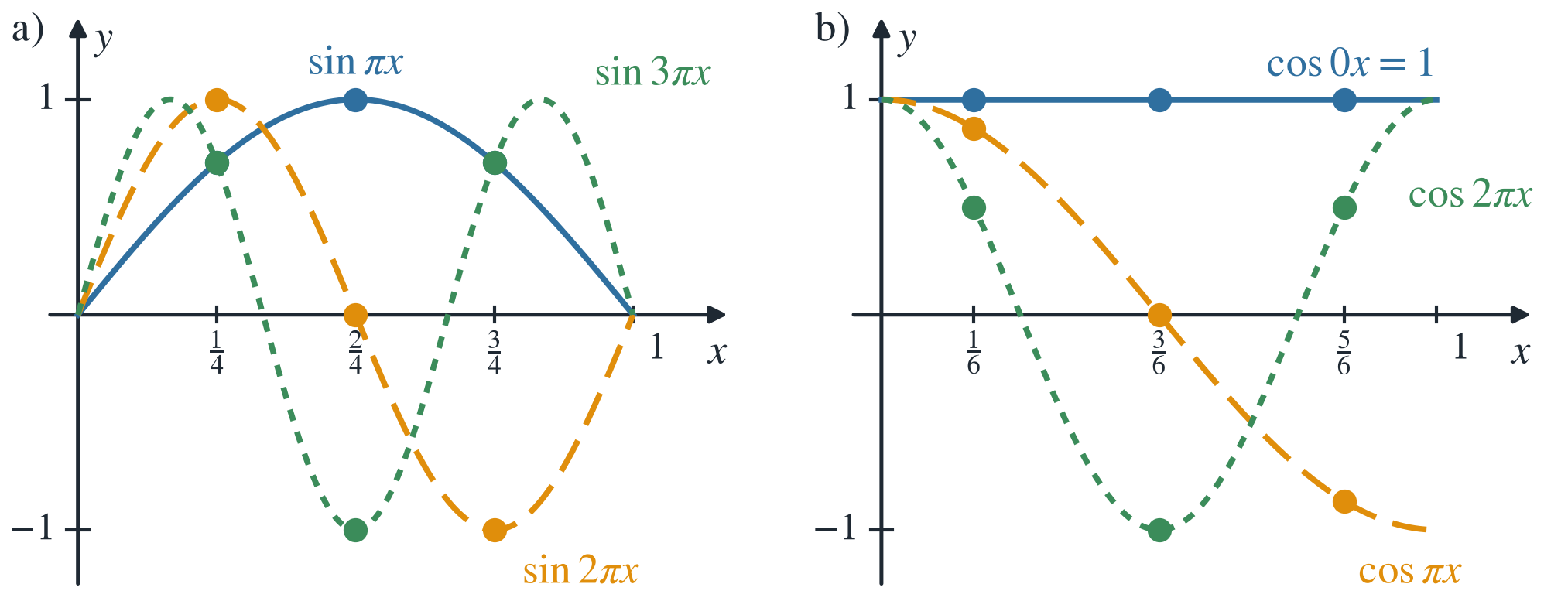
Definition 8.6 (Discrete Sine Transform) The discrete sine transform (DST) is the multiplication by the \(n \times n\) matrix \(\mathrm{DST}\) whose columns are the discrete sine eigenvectors \(v_1, \ldots, v_n\) of the matrix \(K_n\). Its entry in row \(\ell\) and column \(k\) is \(\sin\left(\frac{k\ell\pi}{n+1}\right)\).
For \(n = 3\) the matrix reads
\[ \mathrm{DST} = \begin{pmatrix} \sin\left(\frac{\pi}{4}\right) & \sin\left(\frac{2\pi}{4}\right) & \sin\left(\frac{3\pi}{4}\right) \\ \sin\left(\frac{2\pi}{4}\right) & \sin\left(\frac{4\pi}{4}\right) & \sin\left(\frac{6\pi}{4}\right) \\ \sin\left(\frac{3\pi}{4}\right) & \sin\left(\frac{6\pi}{4}\right) & \sin\left(\frac{9\pi}{4}\right) \end{pmatrix} = \begin{pmatrix} \frac{\sqrt{2}}{2} & 1 & \frac{\sqrt{2}}{2} \\ 1 & 0 & -1\\ \frac{\sqrt{2}}{2} & -1 & \frac{\sqrt{2}}{2} \end{pmatrix}. \]
The columns of the DST matrix are orthogonal vectors of length \(\sqrt{2}\). If we divide all components by \(\sqrt{2}\), the three eigenvectors become orthonormal. Their components lie on sine curves. The DST matrix becomes an orthogonal matrix \(Q = \mathrm{DST}/\sqrt{2}\) with \(Q^{-1} = Q^T\).
We consider the eigenvectors of the matrices \(C_n\). These are sines and cosines, in other words: complex exponentials. The matrices \(C_n\) are even more important than the matrices of the sine and cosine transforms, because the eigenvectors now yield the discrete Fourier transform.
There are no better eigenvectors than these. Every circulant matrix (Definition 8.2) has such eigenvectors (Strang 2010, Ch. 4). Its constant diagonals continue with wrap-around into the next row (the \(-1\) below the main diagonal of \(C_n\) is carried over into the top right corner). Our goal is to determine the eigenvalues and eigenvectors of the matrices \(C_n\). The circulant matrix \(C_4\) has the form \[ C_4 = \begin{pmatrix} 2 & -1 & 0 & -1 \\ -1 & 2 & -1 & 0 \\ 0 & -1 & 2 & -1 \\ -1 & 0 & -1 & 2 \end{pmatrix}. \]
This real symmetric matrix has real, orthogonal eigenvectors (discrete sines and cosines). They have full periods like \(\sin(2k\pi x)\) instead of half periods like \(\sin(k\pi x)\).
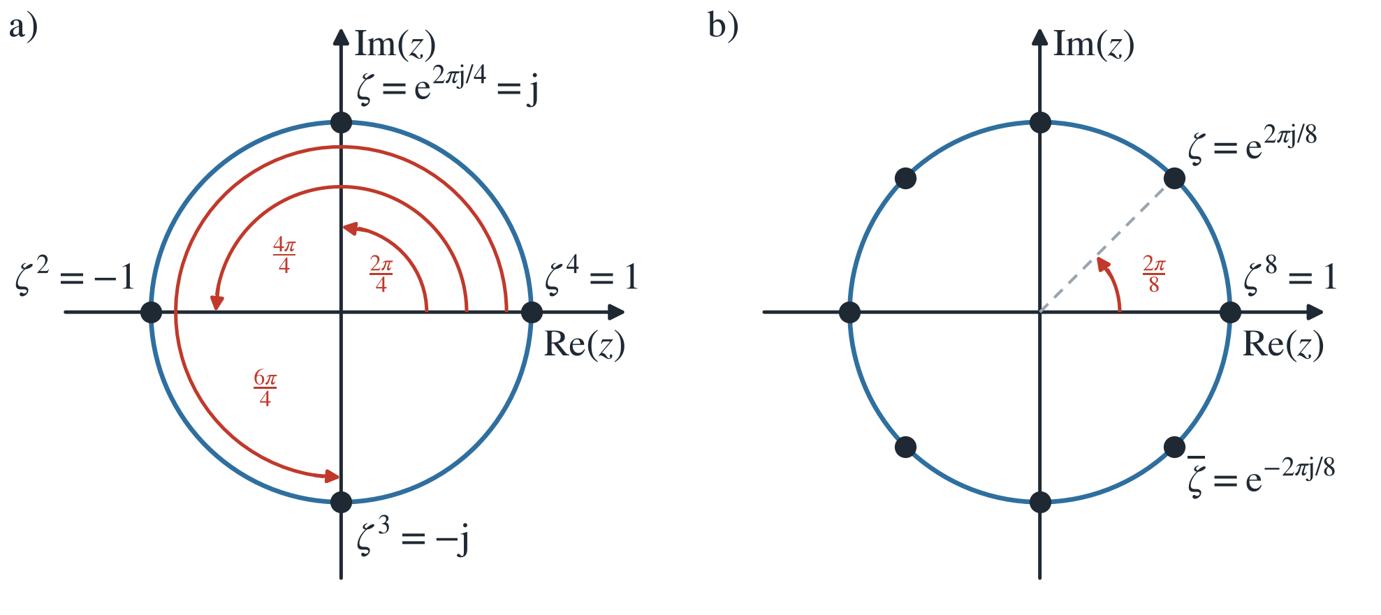
Counting, however, becomes more difficult, because the cosines start with \(k = 0\) and the sines with \(k = 1\). It is better to work with complex exponentials \(\mathrm{e}^{\mathrm{j}\theta}\). The \(k\)th eigenvector of the matrix \(C_n\) arises by sampling the function \(y_k(x) = \mathrm{e}^{\mathrm{j}2\pi kx}\) at the \(n\) grid points \(x = \ell/n\). This brings in the \(n\)th root of unity \(\zeta = \mathrm{e}^{2\pi\mathrm{j}/n}\), a solution of \(z^n = 1\) (Figure 8.2).
Theorem 8.15 (Eigenvectors of the Matrices \(C_n\)) The \(\ell\)th component of the vector \(v_k\) is \[ \mathrm{e}^{\mathrm{j}2\pi k(\ell/n)} = \zeta^{\ell k}, \quad \zeta = \mathrm{e}^{2\pi\mathrm{j}/n} = n\text{th root of unity}. \]
This special number \(\zeta\) is the key to the discrete Fourier transform. Its angle is \(2\pi/n\), which corresponds to the \(n\)th part of the way around the unit circle. The powers of \(\zeta\) move around the unit circle and return to \(\zeta^n = 1\). The eigenvectors and eigenvalues of \(C_n\) are \[ v_k = (1, \zeta^k, \zeta^{2k}, \ldots, \zeta^{(n-1)k}), \qquad \lambda_k = 2 - \zeta^k - \zeta^{-k} = 2 - 2\cos \left(\frac{2\pi k}{n}\right). \]
Theorem 8.16 (Eigenvalues of the Matrix \(C_n\)) Let \(\zeta = \mathrm{e}^{2\pi\mathrm{j}/n}\). For \(k = 0, 1, \ldots, n-1\), the vector \(v_k\) with the components \(\zeta^{\ell k}\), \(\ell = 0, 1, \ldots, n-1\), is an eigenvector of \(C_n\) for the eigenvalue \[ \lambda_k = 2 - \zeta^k - \zeta^{-k} = 2 - 2\cos \left(\frac{2\pi k}{n}\right) = 4\sin^2\left(\frac{\pi k}{n}\right). \]
Proof. Row \(\ell\) of \(C_n v_k\) reads \(-\zeta^{(\ell-1)k} + 2\zeta^{\ell k} - \zeta^{(\ell+1)k} = (2 - \zeta^{-k} - \zeta^{k})\zeta^{\ell k}\). Because \(\zeta^n = 1\), this also holds in the first and the last row, where the indices \(\ell - 1 = -1\) and \(\ell + 1 = n\) are read cyclically as \(n-1\) and \(0\). With \(\zeta^{-k} = \overline{\zeta^k}\) we have \(\zeta^k + \zeta^{-k} = 2\cos(2\pi k/n)\), and \(2 - 2\cos\varphi = 4\sin^2(\varphi/2)\) yields the last form.
The ordering is \(k = 0, 1, \ldots, n-1\). The eigenvector with \(k = 0\) is the constant vector \(v_0 = (1,1,\ldots,1)\). The choice \(k = n\) would give the same vector \((1,1,\ldots,1)\), so nothing new. The smallest eigenvalue \(2 - 2\cos 0\) is \(\lambda_0 = 0\). The matrices \(C_n\) are singular.
The eigenvector with \(k = 1\) is \(v_1 = (1, \zeta, \ldots, \zeta^{n-1})\). Its components are the \(n\) roots of unity, that is, the \(n\) solutions of \(z^n = 1\).
Example 8.4 (Eigenvector \(v_1\) of the Matrix \(C_4\)) Figure 8.2 shows the unit circle \(\lvert z \rvert = 1\) in the complex plane, where in part a) of the figure the \(n = 4\) values are equally spaced around the circle. These numbers are \(\mathrm{e}^0\), \(\mathrm{e}^{2\pi\mathrm{j}/4}\), \(\mathrm{e}^{4\pi\mathrm{j}/4}\), \(\mathrm{e}^{6\pi\mathrm{j}/4}\), and their fourth powers are \(1\). For \(n = 4\), \(\zeta = \mathrm{j}\), and the following holds: \[ C_4 v_1 = \begin{pmatrix} 2 & -1 & 0 & -1 \\ -1 & 2 & -1 & 0 \\ 0 & -1 & 2 & -1 \\ -1 & 0 & -1 & 2 \end{pmatrix} \begin{pmatrix} 1 \\ \mathrm{j} \\ \mathrm{j}^2 \\ \mathrm{j}^3 \end{pmatrix} = (2 - \mathrm{j} - \mathrm{j}^3) \begin{pmatrix} 1 \\ \mathrm{j} \\ \mathrm{j}^2 \\ \mathrm{j}^3 \end{pmatrix} = \lambda_1 v_1. \]
For arbitrary \(n\), the first row gives \(2 - \zeta - \zeta^{n-1} = 2 - \zeta - \overline{\zeta}\). Note that \(\zeta^{n-1}\) is also the complex conjugate \(\overline{\zeta} = \mathrm{e}^{-2\pi\mathrm{j}/n} = 1/\zeta\): multiplying it by \(\zeta\) gives \(1\). Hence \[ \lambda_1 = 2 - \zeta - \overline{\zeta} = 2 - \mathrm{e}^{2\pi\mathrm{j} / n} - \mathrm{e}^{-2\pi\mathrm{j} / n} = 2 - 2\cos \left(\frac{2\pi}{n}\right). \]
Now we know the first two eigenvectors \(v_0 = (1, 1, 1, 1)\) and \(v_1 = (1, \mathrm{j}, \mathrm{j}^2, \mathrm{j}^3)\) of \(C_4\). The eigenvalues are \(0\) and \(2\). To complete the task, we need the eigenvectors \(v_2 = (1, \mathrm{j}^2, \mathrm{j}^4, \mathrm{j}^6)\) and \(v_3 = (1, \mathrm{j}^3, \mathrm{j}^6, \mathrm{j}^9)\). Their eigenvalues are \(4\) and \(2\), which come from \(2 - 2\cos(\pi)\) and \(2 - 2\cos(3\pi/2)\). Then the sum of the eigenvalues is \(0 + 2 + 4 + 2 = 8\), which agrees with the sum of the diagonal entries (the trace \(2+2+2+2\)) of this matrix \(C_4\).
Positive definite matrices (Definition 8.4) have many equivalent characterizations. In my view, we need three basic properties to make progress:
Table 8.2 summarizes the properties of matrices and their eigenvectors. The table contains the most important properties discussed in this section. The eigenvectors of the matrices \(K_n\), \(T_n\), and \(B_n\) are sines and cosines, the eigenvectors of the matrices \(C_n\) are complex exponentials. The last row concerns the singular value decomposition (SVD) \(A = U\Sigma V^T\) of an arbitrary matrix \(A\). Its factors \(U\) and \(V\) are orthogonal, and \(\Sigma\) is diagonal and contains the singular values.
| Matrix | Eigenvalues | Eigenvectors |
|---|---|---|
| symmetric | all \(\lambda\) are real | orthogonal \(v_i^T v_j = 0\) |
| orthogonal | all \(\lvert\lambda\rvert = 1\) | orthogonal \(v_i^T v_j = 0\) |
| skew-symmetric | all \(\lambda\) are imaginary | orthogonal \(v_i^T v_j = 0\) |
| complex Hermitian | all \(\lambda\) are real | orthogonal \(v_i^T v_j = 0\) |
| positive definite | all \(\lambda > 0\) | orthogonal |
| Markov | \(\lambda_{\max} = 1\) | steady state \(v > 0\) |
| similar (Definition 5.2) | \(\lambda(B) = \lambda(A)\) | \(v(B) = Pv(A)\) |
| projection | \(\lambda = 1; 0\) | column space; nullspace |
| reflection \(E - 2uu^T\), \(\lVert u \rVert = 1\) | \(\lambda = -1; 1, \dots, 1\) | \(u\); orthogonal to \(u\) |
| rank 1, \(uv^T\) | \(\lambda = v^T u; 0, \dots, 0\) | \(u\); orthogonal to \(v\) |
| inverse | \(1/\lambda(A)\) | eigenvectors of \(A\) |
| shift by a multiple of \(E\) | \(\lambda(A)\) plus the shift | eigenvectors of \(A\) |
| stable powers | all \(\lvert\lambda\rvert < 1\) | - |
| stable exponential | all \(\operatorname{Re} \lambda < 0\) | - |
| cyclic | \(\lambda_k = \mathrm{e}^{2\pi\mathrm{j}k/n}\) | \(v_k = (1, \lambda_k, \ldots, \lambda_k^{n-1})\) |
| Toeplitz (\(K_n\)) | \(\lambda_k = 2-2\cos \frac{k\pi}{n+1}\) | \(v_k = (\sin \frac{k\pi}{n+1},\sin \frac{2k\pi}{n+1}, \ldots)\) |
| diagonalizable | diagonal of \(\Lambda\) | columns of \(V\) are independent |
| symmetric | diagonal of \(\Lambda\) (real) | columns of \(Q\) are orthonormal |
| Jordan | diagonal of \(J\) | each block gives \(v = (0, \ldots, 1, \ldots, 0)\) |
| SVD | singular values in \(\Sigma\) | eigenvectors of \(A^TA\), \(AA^T\) in \(V, U\) |
This section refers to Chapter 2.1 in Strang (2010).
Figure 8.3 shows three masses \(m_1\), \(m_2\), \(m_3\) connected by springs. In one example it is a chain of four springs, fixed at the top and at the bottom. In the second example there are only three springs: the first spring is fixed at the top, and the lowest mass hangs free. The boundary conditions in the two examples are fixed-fixed and fixed-free, respectively. We seek equations for the essential variables, the displacements of the masses and the tensions in the springs:
\[ u = (u_1, u_2, u_3) = \text{displacements of the masses}, \] \[ w = (w_1, w_2, w_3, w_4) \text{ or } (w_1, w_2, w_3) = \text{tension in the springs}. \]
The displacement of a mass has a positive sign when the mass is pulled downward. Under tension the spring force \(w_i\) has a positive sign, under compression a negative one (\(w_i < 0\)). Under tension the spring is stretched and then pulls the masses together. Under compression the masses are pushed apart by the spring.
We need the elastic properties (the spring constants \(c_i\)) of each spring. This is an essential change compared with Section 8.1! The matrices \(K_n\) and \(T_n\) treated there had “spring constants = 1”. Here \(c_i\) relates the elongation \(e_i\) to the force \(w_i\). Hooke’s law reads \(w_i = c_i e_i\), that is, force equals spring constant times elongation. With four springs there are four constants \(c_1\), \(c_2\), \(c_3\), \(c_4\).
Our task is to link these equations for the individual springs into a vector equation \(f = Ku\) for the whole system. The vector \(f\) is the external force. Gravity pulls on each mass and gives \(f = (m_1g, m_2g, m_3g)\). At the surface of the earth, \(g\) is about \(9.8\,\text{m/s}^2\). Multiplied by the mass, this gives a force.
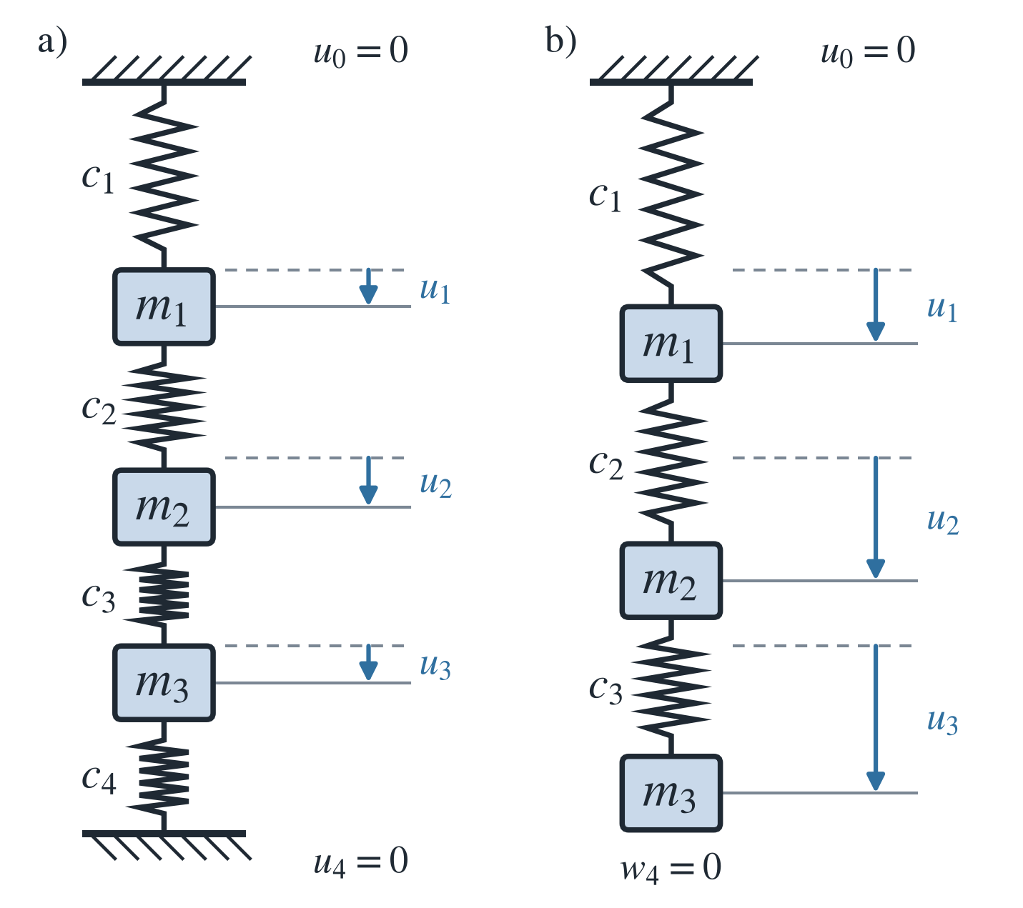
Our real problem is the stiffness matrix \(K\) that links \(u\) to \(f\). Two different structures, namely the springs with fixed-fixed and with fixed-free boundary conditions, also produce two different \(K\).
It is best to construct \(K\) in three steps rather than in one. Now comes the dominant basic pattern of this chapter, which we first look at for a spring chain. Instead of linking the displacements \(u\) directly to the forces \(f\), for \(n\) masses and \(r\) springs it is better to link each vector to its successor in the following list:
The basic pattern that links \(u\), \(e\), \(w\), and \(f\) is shown in Figure 8.4.
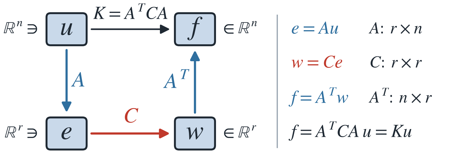
For both examples we will write down the matrices \(A\), \(C\), and \(A^T\), first for the case with fixed ends and then for the case with a freely hanging lower end. Forgive the simplicity of the matrices; their significance lies in their form.
In the first step we determine the elongation \(e\). It is a measure of the strain, that is, of how strongly the springs are stretched. Initially there is no displacement and no stretching (the system lies on a table). When it is set upright, gravity acts. The masses fall by \(u_1\), \(u_2\), \(u_3\). If mass 2 falls by \(u_2\) and mass 1 falls by \(u_1\), then the spring stretches by \(u_2 - u_1\) (Figure 8.5).
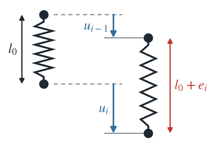
The lower end of spring \(i\) moves down by \(u_i\). Its upper end moves down by \(u_{i-1}\). If both ends move by the same amount, the spring is not stretched: \(u_i = u_{i-1}\) and \(e_i = 0\). Note that the equation \(e_i = u_i - u_{i-1}\) (the difference of displacements) also holds at the ends if we fix them at the top and bottom by \(u_0 = 0\) and \(u_4 = 0\).
In the four equations, the matrix \(A\) is a \(4 \times 3\) difference matrix. We write these four differences \(u_i - u_{i-1}\) as a matrix \(A\) multiplied by a vector \(u\). Our equation for the strain is \(e = Au\): \[ \begin{pmatrix} e_1 \\ e_2 \\ e_3 \\ e_4 \end{pmatrix} = \begin{pmatrix} 1 & 0 & 0 \\ -1 & 1 & 0 \\ 0 & -1 & 1 \\ 0 & 0 & -1 \end{pmatrix} \begin{pmatrix} u_1 \\ u_2 \\ u_3 \end{pmatrix} = \begin{pmatrix} u_1 \\ u_2 - u_1 \\ u_3 - u_2 \\ -u_3 \end{pmatrix}. \]
For a continuous problem, the differences \(e = Au\) become \(e = \frac{\mathrm{d}u}{\mathrm{d}x}\). The matrix becomes a derivative! Instead of a matrix equation we now obtain an ODE.
In the second step, the physical equation \(w = Ce\) links the elongations \(e\) of the springs to the spring tensions \(w\). This is Hooke’s law \(w_i = c_i e_i\) for each individual spring. It is the “constitutive law”, which depends on the material of the spring and on its shape. A soft thin spring has a small \(c_i\), so that a moderate force \(w_i\) can cause a large elongation \(e_i\). Note again that Hooke’s law is linear. This description is nearly exact over a wide range, until the spring is overstretched and the material deforms.
Each spring has its own law. Therefore, the matrix \(C\) in \(w = Ce\) is a diagonal matrix. For the four springs, Hooke’s law in matrix form reads \[ \begin{pmatrix} w_1 \\ w_2 \\ w_3 \\ w_4 \end{pmatrix} = \begin{pmatrix} c_1 & 0 & 0 & 0 \\ 0 & c_2 & 0 & 0 \\ 0 & 0 & c_3 & 0 \\ 0 & 0 & 0 & c_4 \end{pmatrix} \begin{pmatrix} e_1 \\ e_2 \\ e_3 \\ e_4 \end{pmatrix} = Ce. \]
If we substitute \(e = Au\) into \(w = Ce\), we know the relation \(w = CAu\) between the internal spring forces \(w\) and the mass displacements \(u\).
In the third step we come to the balance equation. The internal forces \(w\) of the springs must balance the external forces \(f\) on the masses. Each mass is in equilibrium: it is pulled upward by a spring force \(w_j\) and at the same time pulled downward by a spring force \(w_{j+1}\) and the gravitational force \(f_j\). Hence \(w_j = w_{j+1} + f_j\), or \(f_j = w_j - w_{j+1}\).
The force balance \(A^T w = f\) reads \[ \begin{pmatrix} f_1 \\ f_2 \\ f_3 \end{pmatrix} = \begin{pmatrix} w_1 - w_2 \\ w_2 - w_3 \\ w_3 - w_4 \end{pmatrix} = \begin{pmatrix} 1 & -1 & 0 & 0 \\ 0 & 1 & -1 & 0 \\ 0 & 0 & 1 & -1 \end{pmatrix} \begin{pmatrix} w_1 \\ w_2 \\ w_3 \\ w_4 \end{pmatrix}. \]
This is the matrix \(A^T\)! The balance equation of the forces is \(f = A^T w\). In a natural way, the rows and columns of the \(e\)-\(u\) matrix are transposed so that the \(f\)-\(w\) matrix comes out. Herein lies the beauty of this basic pattern: \(A^T\) appears together with \(A\).
All large finite element programs devote considerable effort to assembling the stiffness matrix \(K = A^TCA\) from smaller pieces. For four springs we do this by matrix multiplication of \(A^T\) with \(CA\). Here is the stiffness matrix \(K\) for fixed-fixed boundary conditions:
\[ K = A^TCA = \begin{pmatrix} 1 & -1 & 0 & 0 \\ 0 & 1 & -1 & 0 \\ 0 & 0 & 1 & -1 \end{pmatrix} \begin{pmatrix} c_1 & 0 & 0 \\ -c_2 & c_2 & 0 \\ 0 & -c_3 & c_3 \\ 0 & 0 & -c_4 \end{pmatrix} = \begin{pmatrix} c_1 + c_2 & -c_2 & 0 \\ -c_2 & c_2 + c_3 & -c_3 \\ 0 & -c_3 & c_3 + c_4 \end{pmatrix}. \]
If all springs are identical with \(c_1 = c_2 = c_3 = c_4 = 1\), then \(C\) is the identity matrix, \(C = E\), and the stiffness matrix reduces to \(K = A^TA\). With \(c_i = 1\) we thus obtain the special matrix \(K_3\):
Theorem 8.17 (Stiffness Matrix with \(C=E\) (Fixed-Fixed)) The stiffness matrix with \(C=E\) is \(K_3\):
\[ K_3 = A^T A = \begin{pmatrix} 2 & -1 & 0 \\ -1 & 2 & -1 \\ 0 & -1 & 2 \end{pmatrix}. \]
A chain of four identical springs, fixed at both ends, has led us to our favorite matrix. A chain of \(n+1\) identical springs would give \(K_n\). The matrix is tridiagonal because each spring is connected only to its two neighbors. It has constant diagonal entries because all springs are identical. The matrix \(K_n\) is symmetric positive definite because nature insists on this property (by producing \(A\) and \(A^T\)).
\(K_3 = A^TA\) is something quite different from \(K_3 = LL^T\). The matrix \(A\) from the problem with four springs is a \(4 \times 3\) matrix. The matrix \(L\) from elimination (Cholesky factorization) is square. The matrix \(K\) is assembled from \(A^TA\) and then factored into \(LL^T\). One step belongs to applied mathematics, the other lies in the realm of scientific computing. Every matrix \(K_n\) is assembled from rectangular matrices and factored into square matrices.
Let me list a few properties of the matrix \(K = A^TCA\). Almost all of them are familiar to you:
This last property has an important consequence for \(u = K^{-1}f\): if all forces act downward (\(f_j > 0\)), then the masses are displaced only downward (\(u_j > 0\)). Bear in mind that the “positivity” of a matrix is something different from its “positive definiteness”. Here the matrix \(K\) is not positive (its entries include \(-1\)), while both matrices \(K\) and \(K^{-1}\) are positive definite.
Example 8.5 (Spring Chain with Fixed-Fixed Ends (Example 2.1 from Strang (2010))) Suppose \(c_i = c\) and \(m_j = m\). Determine the displacements \(u\) and the forces \(w\).
All springs and masses are identical. But the displacements, elongations, and spring forces will not all be identical. The inverse matrix \(K^{-1}\) contains the factor \(\frac{1}{c}\), because the matrix \(K = A^TCA\) contains the factor \(c\). For the displacements, \[ u = K^{-1}f = \frac{1}{4c} \begin{pmatrix} 3 & 2 & 1 \\ 2 & 4 & 2 \\ 1 & 2 & 3 \end{pmatrix} \begin{pmatrix} mg \\ mg \\ mg \end{pmatrix} = \frac{mg}{c} \begin{pmatrix} 1.5 \\ 2.0 \\ 1.5 \end{pmatrix}. \]
The displacement \(u_2\) of the middle mass is larger than \(u_1\) and \(u_3\). The units are consistent: the force \(mg\) divided by the force per unit length \(c\) gives a length \(u\). The elongations of the springs are \[ e = Au = \begin{pmatrix} 1 & 0 & 0 \\ -1 & 1 & 0 \\ 0 & -1 & 1 \\ 0 & 0 & -1 \end{pmatrix} \frac{mg}{c} \begin{pmatrix} 1.5 \\ 2.0 \\ 1.5 \end{pmatrix} = \frac{mg}{c} \begin{pmatrix} 1.5 \\ 0.5 \\ -0.5 \\ -1.5 \end{pmatrix}. \]
The sum of these elongations should be zero because the ends of the chain are fixed. And indeed \(u_1 + (u_2 - u_1) + (u_3 - u_2) + (-u_3) = 0\). To compute the spring force \(w\), by Hooke’s law only \(e\) needs to be multiplied by \(c\). So \(w_1, w_2, w_3, w_4\) equal \(1.5\,mg\), \(0.5\,mg\), \(-0.5\,mg\), \(-1.5\,mg\). The two upper springs are stretched, the two lower springs are compressed.
Note how \(u, e, w\) were computed in this order. We assembled \(K = A^TCA\) from rectangular matrices. To determine \(u = K^{-1}f\), we work with the whole matrix and not with its three parts. The rectangular matrices \(A\) and \(A^T\) have no (two-sided) inverses. In general, you therefore cannot write \(K^{-1} = A^{-1}C^{-1}(A^T)^{-1}\).
The matrices are linked by the triple product \(A^TCA\) and cannot simply be separated again. In general, \(A^Tw = f\) has many solutions. Four equations in three unknowns would usually have no solution. But \(A^TCA\) delivers the correct solution to all three equations in the basic pattern. Only in the case \(r = n\) with square matrices can we go from \(w = (A^T)^{-1}f\) via \(e = C^{-1}w\) to \(u = A^{-1}e\). We will look at this now.
Let us remove the fourth spring. All matrices become \(3 \times 3\) matrices. The pattern does not change! The matrix \(A\) loses its fourth row (there is no \(e_4\)). Furthermore, the matrix \(A^T\) loses its fourth column (there is no \(w_4\)). The stiffness matrix becomes a product of square matrices:
\[ A = \begin{pmatrix} 1 & 0 & 0 \\ -1 & 1 & 0 \\ 0 & -1 & 1 \end{pmatrix}, \quad C = \begin{pmatrix} c_1 & 0 & 0 \\ 0 & c_2 & 0 \\ 0 & 0 & c_3 \end{pmatrix}, \quad A^T = \begin{pmatrix} 1 & -1 & 0 \\ 0 & 1 & -1 \\ 0 & 0 & 1 \end{pmatrix}. \]
For fixed-free boundary conditions, this gives \[ K = A^TCA = \begin{pmatrix} c_1+c_2 & -c_2 & 0 \\ -c_2 & c_2 +c_3 & -c_3 \\ 0 & -c_3 & c_3 \end{pmatrix}. \]
You recognize this matrix in the standard case \(c_1 = c_2 = c_3 = 1\). It is the familiar tridiagonal matrix with the entries \(-1, 2, -1\), but the last entry is not \(c_3 + c_4 = 2\) but \(c_3 = 1\). Compared with \(T_3\) from Section 8.1, the ends are interchanged, so that the hanging matrix \(H_3\) results. This corresponds to a second difference matrix with \(u_0 = 0\) at one end and \(u_4 = u_3\) at the other. The lowest mass hangs free.
Example 8.6 (Fixed-Free Spring Chain (Example 2.2 from Strang (2010))) For the fixed-free hanging spring chain, \(c_i = c\) and \(m_j = m\) for all \(i\) and \(j\). Then
\[ A^TCA = c \begin{pmatrix} 2 & -1 & 0 \\ -1 & 2 & -1 \\ 0 & -1 & 1 \end{pmatrix}, \quad (A^TCA)^{-1} = \frac{1}{c} \begin{pmatrix} 1 & 1 & 1 \\ 1 & 2 & 2 \\ 1 & 2 & 3 \end{pmatrix}. \]
The displacements \(u = K^{-1}f\) differ from those in the example with fixed-fixed boundary conditions because the matrix \(K\) has changed: \[ u = (A^TCA)^{-1}f = \frac{1}{c} \begin{pmatrix} 1 & 1 & 1 \\ 1 & 2 & 2 \\ 1 & 2 & 3 \end{pmatrix} \begin{pmatrix} mg \\ mg \\ mg \end{pmatrix} = \frac{mg}{c} \begin{pmatrix} 3 \\ 5 \\ 6 \end{pmatrix}. \]
In this case with fixed-free boundary conditions, the displacements \((3,\, 5,\, 6)\) are larger than the displacements \((1.5,\, 2.0,\, 1.5)\) from before. The number \(3\) appears as the first displacement \(u_1\) because all three masses pull the first spring downward. The next mass has an additional displacement \((3 + 2 = 5)\) due to the two masses below it. The third mass moves down even further, namely by \((3 + 2 + 1 = 6)\). The elongations \(e = Au\) of the three springs show these three numbers \(3, 2, 1\): \[ e = Au = \begin{pmatrix} 1 & 0 & 0 \\ -1 & 1 & 0 \\ 0 & -1 & 1 \end{pmatrix} \frac{mg}{c} \begin{pmatrix} 3 \\ 5 \\ 6 \end{pmatrix} = \frac{mg}{c} \begin{pmatrix} 3 \\ 2 \\ 1 \end{pmatrix}. \]
After multiplication by \(c\), the forces in the three springs are therefore \(w_1 = 3mg\), \(w_2 = 2mg\), and \(w_3 = mg\). The first spring carries three masses, the second spring two, and the third spring one. All springs are now stretched.
The special feature of a square matrix \(A\) is that the internal forces \(w\) can be read off directly from the external forces \(f\). The balance equation \(A^Tw = f\) determines \(w\) immediately and uniquely, because \(r = n\) and \(A^T\) is square and invertible. For the spring forces, \[ w = (A^T)^{-1} f = \begin{pmatrix} 1 & 1 & 1 \\ 0 & 1 & 1 \\ 0 & 0 & 1 \end{pmatrix} \begin{pmatrix} mg \\ mg \\ mg \end{pmatrix} = \begin{pmatrix} 3mg \\ 2mg \\ mg \end{pmatrix}. \]
Then the elongations \(e\) follow from \(C^{-1}w\) and the displacements \(u\) from \(A^{-1}e\). In this “determinate” case \(r = n\) we may write \((A^TCA)^{-1} = A^{-1}C^{-1}(A^T)^{-1}\).
If the displacement at the upper end is fixed by \(u_0 = 0\), a force is needed to accomplish this. This is an external reaction force \(f_0\) that supports the chain of springs. This reaction force is not given in advance. It is part of the result of the force balance at the upper end. The first spring pulls downward with an internal force \(w_1 = 3mg\). The reaction force pulls upward with \(f_0 = -3mg\) to balance this force. A structural engineer must know the reaction forces to make sure that the support holds and the building does not collapse.
Example 8.7 (Spring Chain with Free-Free Ends (Example 2.3 from Strang (2010))) A spring chain with free-free boundary conditions has no support. This causes trouble with \(A\) and \(K\) (spring 1 has disappeared). The matrix \(A\) is a \(2 \times 3\) matrix, short and wide. Here is \(e = Au\):
\[ e_2 = u_2 - u_1, \quad e_3 = u_3 - u_2, \] \[ \begin{pmatrix} e_2 \\ e_3 \end{pmatrix} = \begin{pmatrix} -1 & 1 & 0 \\ 0 & -1 & 1 \end{pmatrix} \begin{pmatrix} u_1 \\ u_2 \\ u_3 \end{pmatrix}. \]
Now there is a nonzero solution to \(Au = 0\). The masses can move without stretching the springs: the whole chain can move by \(u = (1, 1, 1)\), and still \(e = (0, 0)\). The columns of \(A\) are dependent, and the vector \((1,1,1)\) lies in the nullspace. For this rigid-body motion, \[ u = \begin{pmatrix}1\\1\\1\end{pmatrix}, \quad Au = \begin{pmatrix}0\\0\end{pmatrix} = e. \]
In this case \(A^TCA\) cannot be invertible. \(K\) must be singular, because \(Au = 0\) obviously leads to \(A^TCAu = 0\). The stiffness matrix is still square and symmetric, but it is only positive semidefinite (like \(B_n\) with two free ends): \[ A^TCA = \begin{pmatrix} c_2 & -c_2 & 0 \\ -c_2 & c_2+c_3 & -c_3 \\ 0 & -c_3 & c_3 \end{pmatrix}. \]
The pivots are \(c_2\) and \(c_3\). There is no third pivot. Two eigenvalues are positive, but the vector \((1, 1, 1)\) is an eigenvector for \(\lambda = 0\). The matrix is not invertible, and we can solve \(A^TCAu = f\) only for special vectors \(f\). The external forces must add up to zero: \(f_1 + f_2 + f_3 = 0\). Otherwise, the whole spring chain (with two free ends) would take off like a rocket.
In Strang (2010, Problem 2.1.4, p. 126), the upper end is pulled upward and the lower end downward, with the forces canceling each other. We can solve \(A^TCAu = (-1, 0, 1)\) even though the system is singular. A circle of springs (\(K\) is then the circulant matrix \(C_n\) from Section 8.1) is also singular.
This section refers to Chapter 2.2 in Strang (2010).
This section deals with the most important law of mechanics, Newton’s law \(F = m\ddot{u}\): force equals mass times acceleration. Let \(n\) masses \(m_1, \ldots, m_n\) be given that obey this law. Their displacements \(u_1(t), \ldots, u_n(t)\) change with time, but by no means at nearly the speed of light (we hope). The acceleration of each mass is the second derivative \(\ddot{u} = \frac{\mathrm{d}^2u}{\mathrm{d}t^2}\) (also written as \(u_{tt}\) or \(u''\)). We need the forces \(F\).
Compare the statement of \(F = m\ddot{u}\) with the statement about equilibrium in the previous section. There the masses did not move (\(\ddot{u} = 0\)). Each mass was in equilibrium between external forces \(f\) and spring forces \(Ku\). Now the masses are out of this equilibrium: \(F = f - Ku \neq 0\), the masses are in motion. In the case \(f = 0\) there are only spring forces, and \[M\ddot{u} = -Ku.\]
Friction and damping terms would involve the velocities \(\dot{u} = \frac{\mathrm{d}u}{\mathrm{d}t}\). This is the case for flow problems (and for many applications in which flows play a role). In this section, only \(\ddot{u}\) occurs and no \(\dot{u}\). Without damping or external forces, the springs oscillate forever. The sum of the kinetic energies \(\frac{1}{2} m \dot{u}^2\) of the masses and the stored energies \(\frac{1}{2} c e^2\) of the springs must be constant.
When we treat coupled ODEs, we naturally use matrices. The vector of \(n\) displacements is \(u(t)\), and we write the masses into a diagonal mass matrix \(M = \operatorname{diag}(m_1, \ldots, m_n)\): \[ u(t) = \begin{pmatrix} u_1(t) \\ \vdots \\ u_n(t) \end{pmatrix}, \qquad M = \begin{pmatrix} m_1 & & 0 \\ & \ddots & \\ 0 & & m_n \end{pmatrix}. \]
The vector of the \(n\) external forces on the masses is \(f(t)\). If \(Ku = f\) holds, the masses are in equilibrium: there are no oscillations. The force in Newton’s law \(F = M\ddot{u}\) is the difference \(F = f - Ku\).
Theorem 8.18 (Newton’s Law) \[F = M\ddot{u}, \quad \text{so} \quad f - Ku = M\ddot{u} \quad \text{or} \quad M\ddot{u} + Ku = f.\]
We do not have to repeat the same steps for every new application. That is the advantage of the basic pattern! Once the matrices \(A\), \(C\), \(K = A^TCA\), and \(M\) are known, the system works by itself. The basic equation \(M\ddot{u} + Ku = 0\) with \(f = 0\) is conservative. We will solve it exactly using the eigenvalues and eigenvectors of \(M^{-1}K\).
In real applications, large problems are solved using finite differences with time steps \(\Delta t\). A key point in scientific computing is the choice between “explicit” and “implicit”. With explicit methods we obtain the new \(M u(t +\Delta t)\) directly.
Let us begin with a mass \(m\) hanging from a spring (with spring constant \(c\)). The upper end is fixed. When the mass moves down by a displacement \(u(t)\), the spring pulls it back up with the force \(-cu(t)\). The spring force has a negative sign because it opposes the displacement. Newton’s law \(m\ddot{u} = -cu\) gives the equation for the one unknown \(u(t)\), \[ m\frac{\mathrm{d}^2u}{\mathrm{d}t^2} + cu = 0 \] with given \(u(0)\) and \(\dot{u}(0)\).
Keep in mind that we are talking here about motion about the equilibrium position. Gravity has already been accounted for. If you wanted to compute the total displacement from the rest position (without any stretching), you would have to add \(mg\) on the right-hand side and the value \(\frac{mg}{c}\) to the solution, the constant value of \(u\) at equilibrium. We measure from the equilibrium point rather than from zero.
The solution \(u(t)\) contains cosines and sines (a second-order equation has two solutions). For \(m = 1\) and \(c = 1\), \(\cos(t)\) and \(\sin(t)\) already satisfy the equation \(\ddot{u} + u = 0\). Otherwise, we need a factor \(\frac{c}{m}\) from the second derivative in the equation, so we multiply \(t\) by the natural angular frequency \(\omega_0 = \sqrt{c/m}\):
Theorem 8.19 (Oscillation Solution) With \(\omega_0 = \sqrt{c/m}\), the solution of \(m\ddot{u} + cu = 0\) reads \[ u(t) = A \cos(\omega_0 t) + B \sin(\omega_0 t). \]
At \(t = 0\) the displacement is \(u(0) = A\). Taking the first derivative of \(u(t)\) gives the velocity. At \(t = 0\) the velocity is \(\dot{u}(0) = B\omega_0\). The initial conditions therefore determine \(A = u(0)\) and \[ B = \frac{\dot{u}(0)}{\omega_0} = \sqrt{\frac{m}{c}} \, \dot{u}(0). \]
The larger \(\omega_0\), the faster the mass oscillates. A small mass on a stiff spring oscillates quickly, like an electron. A large mass hanging from a soft spring oscillates slowly, like a heavy ball on a rubber band.
The potential energy in the one spring is \(\frac{1}{2}cu^2\). The kinetic energy of the one mass is \(\frac{1}{2}m(\dot{u})^2\). With more springs and masses, the potential energy becomes \(\frac{1}{2}e^TCe\). The kinetic energy is then \(\frac{1}{2}\dot{u}^TM\dot{u}\). The total energy (sum of kinetic and potential energy) is constant and equal to its value at time \(t = 0\):
Theorem 8.20 (Energy Conservation) \[ \frac{1}{2}m\dot{u}^2(t) + \frac{1}{2}c u^2(t) = \frac{1}{2}m\dot{u}^2(0) + \frac{1}{2}c u^2(0). \]
Proof. For one spring, the derivative of the total energy is \(m\dot{u}\ddot{u} + c u \dot{u} = \dot{u}\,(m\ddot{u} + cu)\). Because \(m\ddot{u} + cu = 0\), this derivative is zero, so the energy does not change.
Example 8.8 (Fixed-Fixed (Example 2.4 from Strang (2010))) We consider two equal masses \(m_1 = m_2\) and three identical springs: both ends are fixed. The \(2 \times 2\) mass matrix is simply \(M = mE\). We are also already familiar with the \(2 \times 2\) stiffness matrix: \[ \text{Fixed-fixed} \quad K = c\begin{pmatrix} 2 & -1 \\ -1 & 2 \end{pmatrix}, \quad M^{-1}K = \frac{c}{m}\begin{pmatrix} 2 & -1 \\ -1 & 2 \end{pmatrix}. \]
The eigenvalues are \(\lambda_1 = \frac{c}{m}\) and \(\lambda_2 = \frac{3c}{m}\). The eigenvectors are \(v_1 = (1, 1)\) and \(v_2 = (1, -1)\). They are orthogonal with respect to the \(M\) inner product. Here, however, \(M = mE\) and \(M^{-1}K\) are symmetric, so they are orthogonal in the usual sense and \(v_1^Tv_2 = 0\). Substitute \(\lambda_i\) and \(v_i\) into the general solution \[ u(t) = \sum_{i=1}^n \left( A_i \cos(\sqrt{\lambda_i} t) + B_i \sin(\sqrt{\lambda_i} t) \right) v_i \tag{8.3}\] The solution is a combination of the normal modes \(v_1\) and \(v_2\): \[ u(t) = \left( A_1 \cos\left(\sqrt{\frac{c}{m}}\, t\right) + B_1 \sin\left(\sqrt{\frac{c}{m}}\, t\right) \right) \begin{pmatrix} 1 \\ 1 \end{pmatrix} + \left( A_2 \cos\left(\sqrt{\frac{3c}{m}}\, t\right) + B_2 \sin\left(\sqrt{\frac{3c}{m}}\, t\right) \right) \begin{pmatrix} 1 \\ -1 \end{pmatrix}. \]
Part a) of Figure 8.7 shows these two pure oscillations. In \(v_1 = (1, 1)\) the masses oscillate in phase. If they start with the initial conditions \(u_1(0) = u_2(0)\) and \(\dot{u}_1(0) = \dot{u}_2(0)\), they oscillate in phase forever. In \(v_2 = (1, -1)\) the masses oscillate in antiphase (they move in opposite directions). The oscillation is faster because \(\lambda_2\) has the factor 3.
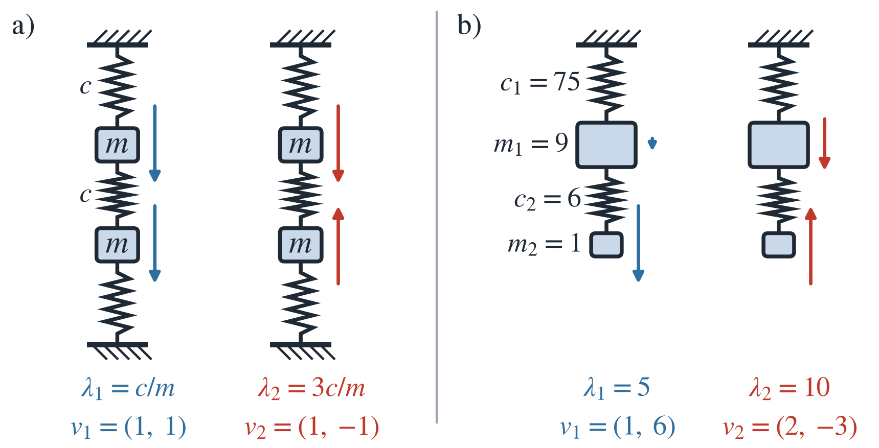
Example 8.9 (Lower End Free (Example 2.5 from Strang (2010))) Masses \(m_1 = 9\), \(m_2 = 1\) with \(c_1 = 75\), \(c_2 = 6\): lower end free.
Now \(c_1 = 75\) and \(c_2 = 6\) are substituted into \(K = A^TCA\). The entries of the last row sum to zero (free end):
\[ \text{Fixed-free} \quad M = \begin{pmatrix} 9 & 0 \\ 0 & 1 \end{pmatrix}, \quad K = \begin{pmatrix} 75+6 & -6 \\ -6 & 6 \end{pmatrix}. \]
The eigenvalues \(\lambda_1 = 5\) and \(\lambda_2 = 10\) come from \(M^{-1}K\) (note the missing symmetry):
\[ M^{-1}K = \begin{pmatrix} 81/9 & -6/9 \\ -6 & 6 \end{pmatrix} \quad \text{leads to} \quad \det\left(M^{-1}K -\lambda E\right) = \lambda^2 - 15\lambda + 50 = 0. \]
The eigenvectors \(v_1 = (1,6)\) and \(v_2 = (2,-3)\) are not orthogonal because \(M^{-1}K\) is not symmetric. We must have \(v_1^TMv_2 = 0\). Here \((1)(9)(2) + (6)(1)(-3) = 0\). Now the smaller mass is displaced more strongly in both normal modes \(v_1\) and \(v_2\), as can be seen in part b) of Figure 8.7. Starting from rest at \(u(0) = (1,0)\) (there are no sine terms), the solution is again a combination of two normal modes:
\[ u(t) = \left( \frac{1}{5} \cos(\sqrt{5} t) + 0 \sin(\sqrt{5}t) \right) \begin{pmatrix} 1 \\ 6 \end{pmatrix} + \left( \frac{2}{5} \cos(\sqrt{10}t) + 0 \sin(\sqrt{10}t) \right) \begin{pmatrix} 2 \\ -3 \end{pmatrix}. \]