import numpy as np
def normalize(x):
    # factor: component of largest magnitude, with its sign,
    # so that a negative dominant eigenvalue is also detected correctly
    fac = x[np.argmax(np.abs(x))]
    x_n = x / fac
return fac, x_n5 Eigenvalues and Eigenvectors
Table 5.1 summarizes the symbols of this chapter together with their type and the place where they are defined.
| Symbol | Meaning | Type | Defined in |
|---|---|---|---|
| \(c\) | Spring constant | Constant | Theorem 2.7 |
| \(c_{12}\) | Spring constant of spring \(i\) (\(c_{12}\): coupling spring) | Constant | Example 5.1 |
| \(i\) | Running index (component, row, eigenvalue number, spring number) | Index | Proposition 5.1 |
| \(k\) | Running index (time/iteration step, mode, eigenvalue number) | Index | Proposition 5.2 |
| \(m\) | Mass | Constant | Theorem 2.6 |
| \(n\) | Order of an ODE; dimension of a matrix or system; number of steps | Index | Definition 5.1 |
| \(t\) | Time | Scalar | Equation 2.8 |
| \(v, v_i\) | Eigenvector; \(v_i\) eigenvector for the eigenvalue \(\lambda_i\) or \(\mu_k\) | Vector | Definition 5.1 |
| \(x_1, x_2\) | Displacement from the rest position; \(x_i\) displacement of mass \(i\); \(x_0\) initial displacement | Function | Theorem 2.7 |
| \(z_k\) | Iteration vector of the power method at step \(k\) (\(z_0\) starting vector) | Vector | Proposition 5.2 |
| \(A\) | Matrix (coefficient, system, or difference matrix, \(e = Au\)) | Matrix | Definition 5.1 |
| \(A_k, Q_k, R_k\) | Matrices in the \(k\)-th step of the QR method | Matrix | Definition 5.3 |
| \(B\) | Further matrix (similar matrix \(A = P^{-1}BP\); \(B = A - \lambda E\) in the brute-force (“Hau-Ruck”) method) | Matrix | Definition 5.2 |
| \(E\) | Identity matrix | Matrix | Definition 5.1 |
| \(P\) | Invertible matrix of a similarity transformation, \(A = P^{-1}BP\) | Matrix | Definition 5.2 |
| \(Q\) | Orthogonal matrix, \(Q^T Q = E\); columns are orthonormal eigenvectors | Matrix | Definition 5.3 |
| \(R\) | Upper triangular matrix of the QR decomposition | Matrix | Definition 5.3 |
| \(T\) | Period of oscillation; \(T_0\) of the simple pendulum, \(T_{\mathrm{d}}\) of the damped oscillation | Scalar | Figure 2.3 |
| \(\gamma_i\) | Coefficient of a linear combination (weights of the RK2 method; expansion of the starting vector in eigenvectors; basis representation in the eigenspace) | Scalar | Equation 3.7 |
| \(\kappa\) | Coupling parameter \(\kappa = c_{12}/m\) of two coupled oscillators | Constant | Example 5.1 |
| \(\lambda, \lambda_i\) | Eigenvalue or root of the characteristic equation (exponent in the ansatz \(\mathrm{e}^{\lambda t}\)); \(\lambda_i\), \(\lambda_k\), \(\lambda_{1,2}\), \(\lambda_{k\pm} = \pm\mathrm{j}\omega_k\) | Scalar | Definition 5.1 |
| \(\tilde{\lambda}_k\) | Eigenvalue of the shifted matrix \(A - \lambda_1 E\) | Scalar | Proposition 5.4 |
| \(\xi_1, \xi_2\) | Components of an unknown eigenvector | Scalar | Example 5.1 |
| \(\pi\) | The number pi (italic, KaTeX exception) | Constant | Figure 2.3 |
| \(\omega\) | Angular frequency (excitation angular frequency; imaginary part of an eigenvalue; frequency of an eigenfunction) | Scalar | Example 5.1 |
| \(\omega_0\) | Natural angular frequency of the undamped single-mass oscillator, \(\omega_0 = \sqrt{c/m}\) (simple pendulum: \(\sqrt{g/l}\)) | Constant | Equation 2.8 |
| \(\omega_1, \omega_2\) | Natural angular frequency of the \(k\)-th normal mode (\(\omega_1, \omega_2\) in 05) | Scalar | Remark 5.1 |
| \(\dot{x}, \ddot{x}\) | First and second derivative with respect to time \(t\) | Operator | Equation 2.8 |
| \(A^T\) | Transpose | Operator | Definition 5.3 |
| \(A^{-1}\) | Inverse | Operator | Proposition 5.3 |
| \(\det\) | Determinant | Operator | Proposition 5.1 |
| \(\lvert \lambda \rvert\) | Euclidean norm, absolute value | Operator | Proposition 5.2 |
| local | \(\varepsilon_i\) (Example 5.3); placeholder \(*\) for arbitrary entries (QR method) | local | where used |
5.1 Definitions
Papula (2015) gives an introduction to the topic in Part I, Linear Algebra, Chapter 7, “Eigenvalues and Eigenvectors of a Square Matrix”.
Definition 5.1 (Eigenvalues and Eigenvectors) Let \(A\) be a (real or complex) matrix of order \(n\) and \(E\) the identity matrix of order \(n\). The matrix equation \[ (A - \lambda E)\, v = 0 \] describes an \(n\)-dimensional eigenvalue problem. A number \(\lambda\) for which this equation has a solution \(v \neq 0\) is called an eigenvalue of the matrix \(A\). Every such solution \(v\) is called an eigenvector of \(A\) for the eigenvalue \(\lambda\). The matrix \(A - \lambda E\) is called the characteristic matrix of \(A\).
The eigenvalues and eigenvectors of the matrix \(A\) can be computed step by step.
Proposition 5.1 (Characteristic Equation) The eigenvalues of \(A\) are the solutions \(\lambda_1, \lambda_2, \ldots, \lambda_n\) of the characteristic equation \[ \det (A - \lambda E) = 0, \] an algebraic equation of degree \(n\). An eigenvector \(v_i\) for the eigenvalue \(\lambda_i\) is a nontrivial solution of the homogeneous linear system of equations \[ (A - \lambda_i E)\, v_i = 0 \quad (i = 1, 2, \ldots, n). \]
Proof. The homogeneous system \((A - \lambda E)\, v = 0\) has a solution \(v \neq 0\) if and only if the matrix \(A - \lambda E\) is singular, that is, if \(\det(A - \lambda E) = 0\).
Eigenvectors are usually given in normalized form. A multiple eigenvalue may have several linearly independent eigenvectors.
Example 5.1 (Normal Modes of Coupled Mechanical Systems) Figure 5.1 shows two identical oscillatory mechanical systems, each consisting of an oscillating mass \(m\) and an elastic spring with spring constant \(c\), which are connected to each other, i.e., coupled, by a coupling spring with spring constant \(c_{12}\).
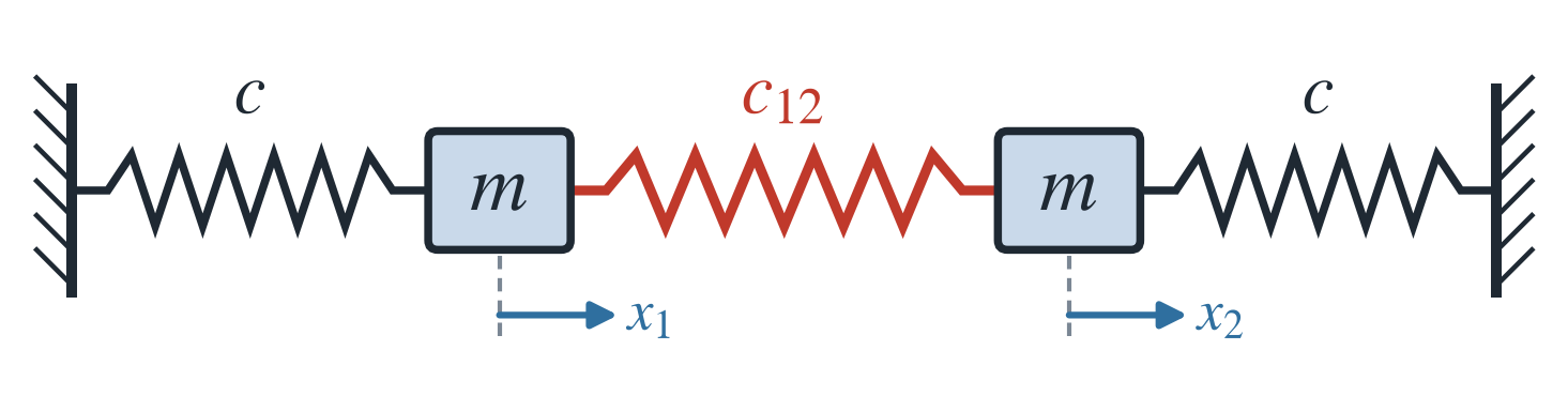
This system is capable of so-called normal modes in the direction of the system axis. Both masses then oscillate harmonically with the same angular frequency \(\omega\). Their position coordinates \(x_1\) and \(x_2\) are therefore periodic functions of time \(t\) with period \(T = 2 \pi / \omega\). The still unknown angular frequencies of these normal modes are the square roots of the (real) eigenvalues of the so-called system matrix \(A\).
The system matrix can be set up from Newton’s second law and Hooke’s law for the spring forces (Theorem 2.6, Theorem 2.7). The first mass is acted on by the spring force \(-c x_1\) and by the force \(-c_{12}(x_1 - x_2)\) of the coupling spring. Its equation of motion is therefore \[ m \ddot{x}_1 = -c x_1 - c_{12}(x_1 - x_2). \] For the second mass one obtains correspondingly \[ m \ddot{x}_2 = - c_{12}(x_2 - x_1) - c x_2. \] Note the signs of the spring forces. Collecting the terms in \(x_1\) and \(x_2\) yields the equations \[ m \ddot{x}_1 = - (c + c_{12}) x_1 + c_{12} x_2 \tag{5.1}\] and \[ m \ddot{x}_2 = c_{12} x_1 - (c + c_{12}) x_2. \tag{5.2}\] Moving all terms to the left-hand side gives the system of equations \[\begin{align} m \ddot{x}_1 + (c + c_{12}) x_1 - c_{12} x_2 & = 0,\\ m \ddot{x}_2 - c_{12} x_1 + (c + c_{12}) x_2 & = 0. \end{align}\] In matrix form it reads \[ m \begin{pmatrix} \ddot{x}_1 \\ \ddot{x}_2 \end{pmatrix} + \begin{pmatrix} c + c_{12} & -c_{12} \\ -c_{12} & c + c_{12} \end{pmatrix} \begin{pmatrix} x_1 \\ x_2 \end{pmatrix} = 0, \] so that we obtain the system matrix \[ A = \begin{pmatrix} (c + c_{12})/m & -c_{12}/m \\ -c_{12}/m & (c + c_{12})/m \end{pmatrix}. \] With the natural angular frequency \(\omega_0 = \sqrt{c/m}\) of the uncoupled spring-mass systems (Equation 2.8) and the coupling parameter \(\kappa = c_{12}/m\), the system matrix can be written as \[ A = \begin{pmatrix} \omega_0^2 + \kappa & -\kappa \\ -\kappa & \omega_0^2 + \kappa \end{pmatrix}. \]
The required eigenvalues follow from the characteristic equation \[ \det (A - \lambda E) = \begin{vmatrix} \omega_0^2 + \kappa - \lambda & -\kappa \\ -\kappa & \omega_0^2 + \kappa - \lambda \end{vmatrix} = (\omega_0^2 + \kappa - \lambda)^2 - \kappa^2 = 0. \] We obtain \[ (\omega_0^2 + \kappa - \lambda)^2 = \kappa^2 \quad \Rightarrow \quad \omega_0^2 + \kappa - \lambda = \pm \kappa \quad \Rightarrow \quad \lambda_{1,2} = \omega_0^2 + \kappa \mp \kappa. \] The eigenvalues of the system matrix \(A\) are therefore \[ \lambda_1 = \omega_0^2 = c/m \tag{5.3}\] and \[ \lambda_2 = \omega_0^2 + 2\kappa = (c + 2c_{12})/m. \tag{5.4}\]
By Proposition 5.1, the eigenvectors \(v_1\) and \(v_2\) for the eigenvalues \(\lambda_1\) and \(\lambda_2\) are the nontrivial solutions of the homogeneous linear systems of equations \((A - \lambda_i E)\, v_i = 0\). We denote the components of the eigenvector to be determined by \(\xi_1\) and \(\xi_2\). For \(\lambda_1 = \omega_0^2\), since \(\omega_0^2 + \kappa - \lambda_1 = \kappa\), we obtain the system of equations \[ \begin{pmatrix} \kappa & -\kappa \\ -\kappa & \kappa \end{pmatrix} \begin{pmatrix} \xi_1 \\ \xi_2 \end{pmatrix} = \begin{pmatrix} 0 \\ 0 \end{pmatrix}. \] Adding the first equation to the second and dividing the first equation by \(\kappa\) gives \[ \begin{pmatrix} 1 & -1 \\ 0 & 0 \end{pmatrix} \begin{pmatrix} \xi_1 \\ \xi_2 \end{pmatrix} = \begin{pmatrix} 0 \\ 0 \end{pmatrix}, \] hence \(\xi_1 = \xi_2\) and thus the eigenvector \(v_1 = \begin{pmatrix} 1 \\ 1 \end{pmatrix}\). Analogously, for \(\lambda_2 = \omega_0^2 + 2\kappa\) we obtain the eigenvector \(v_2 = \begin{pmatrix} 1 \\ -1 \end{pmatrix}\).
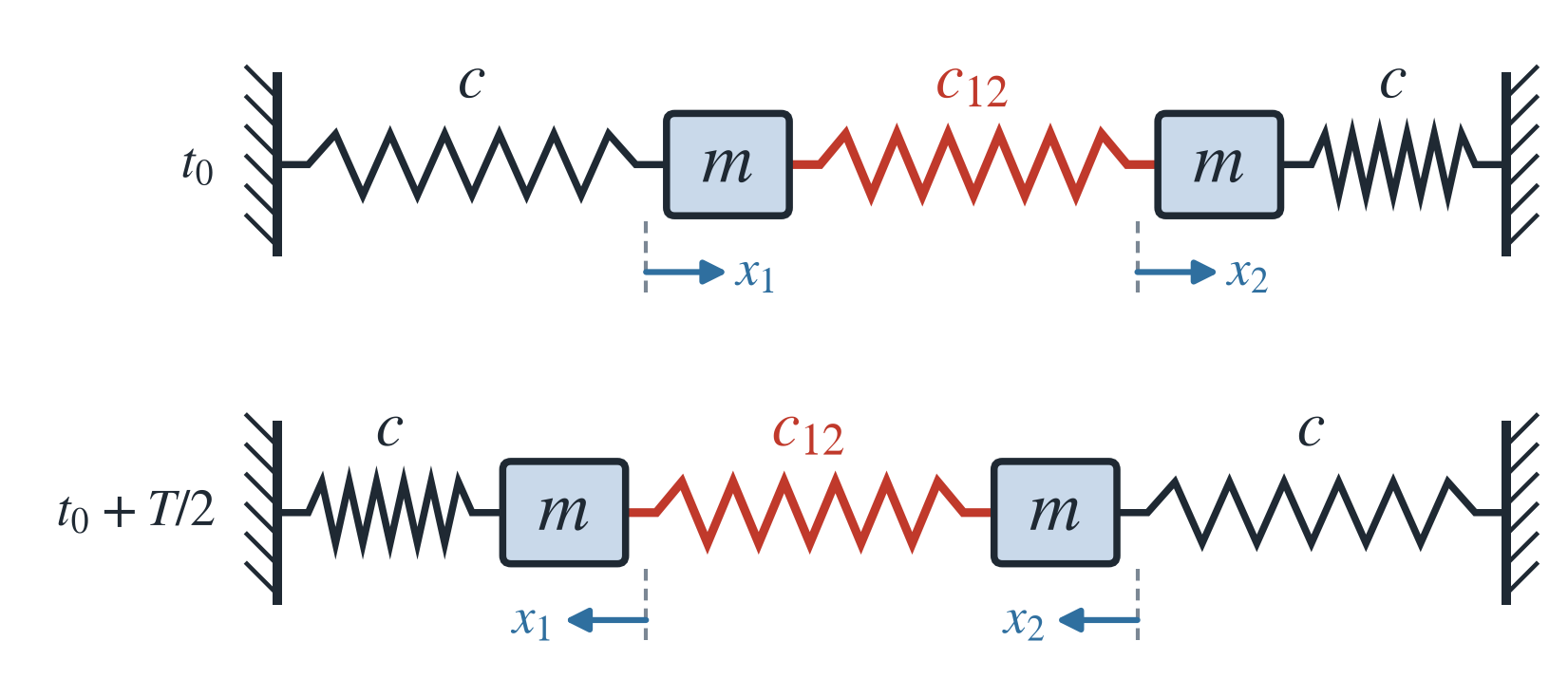
Remark 5.1 (Interpretation of the Eigenvalues and Eigenvectors). Taking square roots in Equation 5.3 and Equation 5.4 yields the angular frequencies of the two normal modes in the direction of the system axis, \[ \omega_1 = \sqrt{c/m} \quad \text{and} \quad \omega_2 = \sqrt{(c + 2c_{12})/m}. \] The first value corresponds to the natural angular frequency \(\omega_0\), i.e., the angular frequency of the uncoupled spring-mass systems: \[ \omega_1 = \omega_0 = \sqrt{c/m}. \] In this normal mode the masses oscillate in phase (eigenvector \(v_1 = \begin{pmatrix} 1 \\ 1 \end{pmatrix}\)). The coupling spring is not loaded, see Figure 5.2.
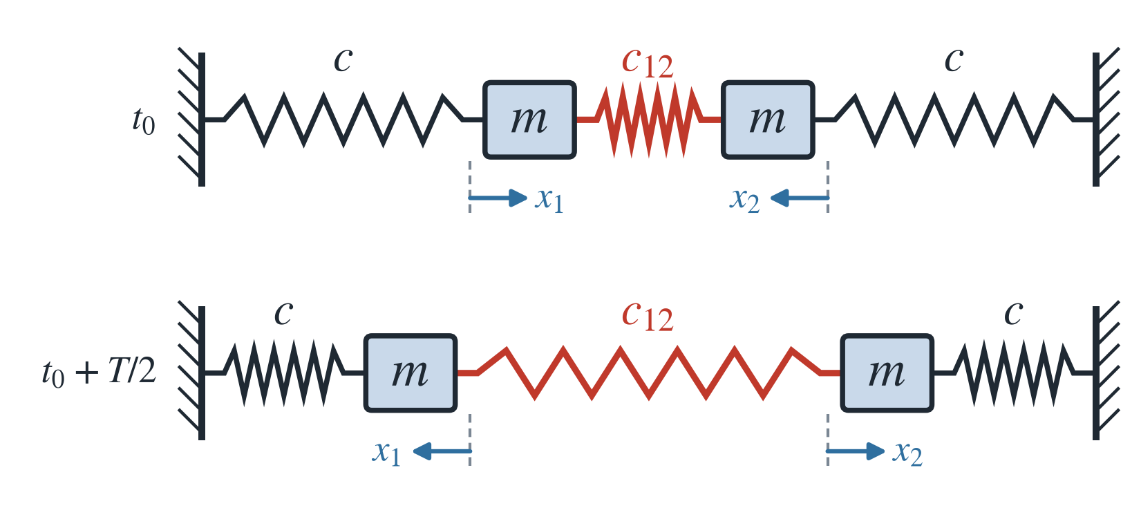
In the second normal mode, with the larger angular frequency \[ \omega_2 = \sqrt{(c + 2c_{12})/m} > \omega_0 = \sqrt{c/m} \] and the eigenvector \(v_2 = \begin{pmatrix} 1 \\ -1 \end{pmatrix}\), the masses instead oscillate in antiphase. The coupling spring is then loaded to the maximum extent, see Figure 5.3.
5.2 Numerical Eigenvalue Computations
5.2.1 The Power Method (Largest Eigenvalue)
5.2.1.1 Derivation
For some problems we only need the eigenvalue of largest magnitude (the dominant eigenvalue) and the corresponding eigenvector. In such cases the power method is suitable, an iterative method that converges to this eigenvalue.
Consider an \(n \times n\) matrix \(A\) with \(n\) real eigenvalues \(\lambda_1, \lambda_2, \dots, \lambda_n\) and \(n\) linearly independent corresponding eigenvectors \(v_1, v_2, \dots, v_n\). Let the eigenvalues be ordered such that \(|\lambda_1| > |\lambda_2| \ge \dots \ge |\lambda_n|\). All that matters is that \(\lambda_1\) is strictly larger in magnitude than all other eigenvalues. These may be equal to one another.
Because the eigenvectors are linearly independent, they form a basis. Every vector in the same space can therefore be written as a linear combination of the eigenvectors, in particular an arbitrary starting vector \(z_0\): \[ z_0 = \gamma_1 v_1 + \gamma_2 v_2 + \dots + \gamma_n v_n. \] We assume \(\gamma_1 \ne 0\). If \(\gamma_1 = 0\), we choose a different starting vector.
Proposition 5.2 (Convergence of the Power Method) Under these assumptions, the vectors \(z_k = A^k z_0 / (\gamma_1 \lambda_1^k)\), \(k = 1, 2, \dots\), satisfy \[ z_k = v_1 + \frac{\gamma_2}{\gamma_1}\left(\frac{\lambda_2}{\lambda_1}\right)^k v_2 + \dots + \frac{\gamma_n}{\gamma_1}\left(\frac{\lambda_n}{\lambda_1}\right)^k v_n \] and \(A z_{k-1} = \lambda_1 z_k\) for \(k \ge 2\). As \(k \to \infty\), \(z_k\) tends to \(v_1\), so \(A z_{k-1} \approx \lambda_1 v_1\) holds for large \(k\).
Proof. We multiply \(z_0\) by \(A\). Since \(A v_i = \lambda_i v_i\), we obtain \[ A z_0 = \gamma_1 A v_1 + \gamma_2 A v_2 + \dots + \gamma_n A v_n = \gamma_1 \lambda_1 v_1 + \gamma_2 \lambda_2 v_2 + \dots + \gamma_n \lambda_n v_n. \] Factoring out \(\gamma_1 \lambda_1\) gives \[ A z_0 = \gamma_1 \lambda_1 \left[v_1 + \frac{\gamma_2}{\gamma_1}\frac{\lambda_2}{\lambda_1}v_2 + \dots + \frac{\gamma_n}{\gamma_1}\frac{\lambda_n}{\lambda_1}v_n\right] = \gamma_1 \lambda_1 z_1. \] This completes the first iteration. Multiplying \(z_1\) by \(A\) starts the second iteration: \[ A z_1 = \lambda_1 v_1 + \frac{\gamma_2}{\gamma_1}\frac{\lambda_2^2}{\lambda_1}v_2 + \dots + \frac{\gamma_n}{\gamma_1}\frac{\lambda_n^2}{\lambda_1}v_n = \lambda_1 \left[v_1 + \frac{\gamma_2}{\gamma_1}\frac{\lambda_2^2}{\lambda_1^2}v_2 + \dots + \frac{\gamma_n}{\gamma_1}\frac{\lambda_n^2}{\lambda_1^2}v_n\right] = \lambda_1 z_2. \] Continuing the multiplication with each new vector, one obtains in the \(k\)-th step \[ A z_{k-1} = \lambda_1 \left[v_1 + \frac{\gamma_2}{\gamma_1}\frac{\lambda_2^k}{\lambda_1^k}v_2 + \dots + \frac{\gamma_n}{\gamma_1}\frac{\lambda_n^k}{\lambda_1^k}v_n\right] = \lambda_1 z_k. \] Since \(\lambda_1\) is the eigenvalue of largest magnitude, \(\left|\lambda_i/\lambda_1\right| < 1\) for all \(i > 1\). For sufficiently large \(k\), \((\lambda_i/\lambda_1)^k\) is therefore close to \(0\) for all \(i > 1\). All terms containing this ratio can be neglected as \(k\) grows: \[ A z_{k-1} \approx \lambda_1 v_1. \]
For sufficiently large \(k\), the power method thus yields the largest eigenvalue and the corresponding eigenvector. In the implementation we normalize the vector in every iteration by factoring out its component of largest magnitude, so that this component equals 1. The normalization factor then yields the largest eigenvalue, and the normalized vector the corresponding eigenvector.
The iteration stops as soon as one of three common criteria is met: the difference between the eigenvalues of successive iterations falls below a tolerance, the angle between successive eigenvectors falls below a threshold, or the norm of the residual vector falls below a prescribed value.
Example 5.2 (Power Method for a \(2 \times 2\) Matrix) The largest eigenvalue of the matrix \[
A = \begin{pmatrix}
0 & 2\\
2 & 3\\
\end{pmatrix}
\] is \(4\). We determine this eigenvalue and its eigenvector numerically with the power method, starting from the starting vector \(z_0 = (1, 1)^T\). In Python the power method can be implemented as follows. The variable x holds the current iteration vector \(z_k\).
x = np.array([1, 1])
A = np.array([[0, 2],
              [2, 3]])

for i in range(8):
    x = np.dot(A, x)
    lambda_1, x = normalize(x)

print(f'Eigenvalue: {lambda_1}')
print(f'Eigenvector: {x}')
Eigenvalue: 3.999949137887188
Eigenvector: [0.50000636 1. ]Example 5.3 (Normalization in the Power Method) We answer two questions about the implementation in Example 5.2: Why is the vector normalized in every iteration? And why does lambda_1 hold the largest eigenvalue after the iteration?
Why normalize? Without normalization, \(z_k = A^k z_0\) after \(k\) steps. By the derivation above, this vector behaves like \(\gamma_1 \lambda_1^k v_1\), so its components grow like \(\lambda_1^k\) (for \(\lvert\lambda_1\rvert > 1\)) or decay like \(\lambda_1^k\) (for \(\lvert\lambda_1\rvert < 1\)). For the matrix from Example 5.2 with \(\lambda_1 = 4\), eight steps without normalization already give \[
A^8 z_0 = \begin{pmatrix} 39322 \\ 78643 \end{pmatrix}.
\] Double-precision floating-point numbers only reach about \(1.8 \cdot 10^{308}\). Since \(4^{512} = 2^{1024} \approx 1.8 \cdot 10^{308}\), the components overflow to inf after roughly 500 steps, and from then on the iteration is worthless. For \(\lvert\lambda_1\rvert < 1\) they underflow to zero accordingly. Normalization prevents both: after every step, the component of largest magnitude equals \(1\). The direction of the vector, which is all that matters for an eigenvector, does not change. Thus \(A^8 z_0\), divided by \(78643\), also equals \((0.500006,\ 1)^T\).
Why does lambda_1 hold the eigenvalue? The function normalize returns the component of largest magnitude of the vector \(A z_{k-1}\) as the factor fac, and this factor is stored in lambda_1. Once the iteration has converged, \(z_{k-1}\) is an eigenvector whose component of largest magnitude equals \(1\). For an eigenvector \(v\) of this form, for instance \[
v =
\begin{pmatrix}
1\\
\varepsilon_1\\
\varepsilon_2\\
\vdots\\
\varepsilon_{n-1}
\end{pmatrix}
\quad \text{with} \quad \lvert\varepsilon_i\rvert \le 1,
\] we have \[
Av = \lambda v =
\begin{pmatrix}
\lambda\\
\lambda\varepsilon_1\\
\lambda\varepsilon_2\\
\vdots\\
\lambda\varepsilon_{n-1}
\end{pmatrix}.
\] The component of largest magnitude of \(Av\) is therefore \(\lambda\) itself, and normalize returns exactly this value as the factor. In the example, \(z_k\) converges to \(v_1 = (0.5,\ 1)^T\), and \[
A v_1 = \begin{pmatrix} 0 & 2\\ 2 & 3 \end{pmatrix} \begin{pmatrix} 0.5 \\ 1 \end{pmatrix} = \begin{pmatrix} 2 \\ 4 \end{pmatrix} = 4 \begin{pmatrix} 0.5 \\ 1 \end{pmatrix}.
\] The normalization factor is \(4 = \lambda_1\), and the normalized vector is again \(v_1\). Since fac keeps the sign of the component, a negative dominant eigenvalue is detected correctly as well.
5.2.2 The Inverse Power Method
Proposition 5.3 (Eigenvalues of the Inverse Matrix) If \(A\) is invertible and \(\lambda\) is an eigenvalue of \(A\) with eigenvector \(v\), then \(1/\lambda\) is an eigenvalue of the inverse matrix \(A^{-1}\) with the same eigenvector \(v\).
Proof. Since \(A\) is invertible, \(\lambda \neq 0\). Multiplying \(Av = \lambda v\) by \(A^{-1}\) gives \(v = \lambda A^{-1} v\), hence \(A^{-1} v = \lambda^{-1} v\).
With Proposition 5.3 and the power method, the eigenvalue of \(A\) with the smallest magnitude can be determined. This is the basis of the inverse power method. Instead of multiplying by \(A\), we multiply by \(A^{-1}\) in every iteration and thus find the eigenvalue \(1/\lambda_n\) of \(A^{-1}\) with the largest magnitude. Its reciprocal \(\lambda_n\) is the eigenvalue of \(A\) with the smallest magnitude.
5.2.3 The Shifted Power Method
In some cases we need all eigenvalues and eigenvectors, not only the largest and the smallest. A simple but inefficient way is the shifted power method. The next section presents a more efficient method.
Proposition 5.4 (Eigenvalues of the Shifted Matrix) If \(A\) has the eigenvalues \(\lambda_1, \dots, \lambda_n\) with the eigenvectors \(v_1, \dots, v_n\), then the shifted matrix \(A - \lambda_1 E\) has the same eigenvectors and the eigenvalues \[ \tilde{\lambda}_k = \lambda_k - \lambda_1, \quad k = 1, \dots, n, \] that is, \(0, \lambda_2 - \lambda_1, \lambda_3 - \lambda_1, \dots, \lambda_n - \lambda_1\).
Proof. From \(A v_k = \lambda_k v_k\) it follows that \((A - \lambda_1 E)\, v_k = (\lambda_k - \lambda_1)\, v_k\).
Applying the power method to the shifted matrix yields its eigenvalue \(\tilde{\lambda}_k\) of largest magnitude. Since \(\tilde{\lambda}_k = \lambda_k - \lambda_1\), this gives the eigenvalue \(\lambda_k = \tilde{\lambda}_k + \lambda_1\) of \(A\). Repeating this procedure several times finds all remaining eigenvalues, albeit at considerable cost. A better method for determining all eigenvalues is the QR method. It is named after the QR decomposition \(A = QR\) of a matrix into an orthogonal matrix \(Q\) and an upper triangular matrix \(R\) (Definition 5.3).
5.2.4 The QR Decomposition
5.2.4.1 Derivation
The QR method is a preferred iterative method for finding all eigenvalues of a matrix (but not the eigenvectors at the same time). It rests on two concepts, the similarity of matrices and the QR decomposition.
Definition 5.2 (Similar Matrices) Two square matrices \(A\) and \(B\) are called similar if there is an invertible matrix \(P\) with \[ A = P^{-1}BP. \]
Proposition 5.5 (Eigenvalues of Similar Matrices) Similar matrices have the same eigenvalues. If \(A = P^{-1}BP\) and \(v\) is an eigenvector of \(B\) for the eigenvalue \(\lambda\), then \(P^{-1}v\) is an eigenvector of \(A\) for the same eigenvalue.
Proof. From \(Bv = \lambda v\) it follows that \(A P^{-1} v = P^{-1} B P P^{-1} v = P^{-1} B v = \lambda P^{-1} v\). Here \(P^{-1} v \neq 0\) because \(P^{-1}\) is invertible. Conversely, since \(B = P A P^{-1}\), every eigenvalue of \(A\) is also an eigenvalue of \(B\).
Definition 5.3 (QR Decomposition) A matrix \(Q\) is called orthogonal if \(Q^{-1} = Q^T\), that is, \(Q^{-1}Q = Q^TQ = E\). The QR decomposition of a matrix \(A\) is its representation \(A = QR\) as the product of an orthogonal matrix \(Q\) and an upper triangular matrix \(R\).
How do we link these two concepts to find the eigenvalues? Let \(A_0\) be a matrix whose eigenvalues are to be determined. In the \(k\)-th step (starting with \(k = 0\)) we decompose \(A_k = Q_kR_k\), where \(Q_k\) is an orthogonal matrix and \(R_k\) is an upper triangular matrix. We then form \(A_{k+1} = R_kQ_k\). Then \[ A_{k+1} = R_kQ_k = Q^{-1}_kQ_kR_kQ_k = Q^{-1}_kA_kQ_k. \] By Definition 5.2 (with \(P = Q_k\)), all \(A_k\) are therefore similar and, by Proposition 5.5, have the same eigenvalues. As the iteration proceeds, the \(A_k\) eventually converge to an upper triangular matrix \[ A_{k+1} = R_kQ_k = \begin{pmatrix} \lambda_1 & * & \dots & *\\ 0 & \lambda_2 & \dots & *\\ & & \dots &\\ 0 & 0 & \dots & \lambda_n\\ \end{pmatrix}, \] whose diagonal elements are the eigenvalues of the matrix. Here \(*\) stands for arbitrary entries.
In every iteration of the QR method, the matrix can be factored into an orthogonal and an upper triangular matrix using a special matrix, the Householder matrix. We do not go into the mathematical details of how to obtain \(Q\) and \(R\) from the matrix. Instead, we directly use the Python function that returns both matrices.
5.2.4.2 The QR Method: Implementation in Python
Example 5.4 (QR Method for a \(2 \times 2\) Matrix) We use the function qr from numpy.linalg to decompose the matrix \[
A = \begin{pmatrix}
0 & 2\\
2 & 3\\
\end{pmatrix}.
\] We first import the required libraries and then perform the QR decomposition of \(A\). The variables q and r hold the factors \(Q\) and \(R\).
import numpy as np
from numpy.linalg import qr
A = np.array([[0, 2],
              [2, 3]])

q, r = qr(A)

print('Q:', q)
print('R:', r)

b = np.dot(q, r)
print('QR:', b)
Q: [[ 0. -1.]
[-1. 0.]]
R: [[-2. -3.]
[ 0. -2.]]
QR: [[0. 2.]
[2. 3.]]Next, we apply the QR method to find the eigenvalues of the matrix.
A = np.array([[0, 2],
              [2, 3]])
for i in range(20):
    q, r = qr(A)
    A = np.dot(r, q)
    if (i+1) % 5 == 0:
        print(f'Iteration {i+1}: {A}')
Iteration 5: [[ 3.99998093 0.00976559]
[ 0.00976559 -0.99998093]]
Iteration 10: [[ 4.00000000e+00 9.53674316e-06]
[ 9.53674316e-06 -1.00000000e+00]]
Iteration 15: [[ 4.00000000e+00 9.31322576e-09]
[ 9.31322575e-09 -1.00000000e+00]]
Iteration 20: [[ 4.00000000e+00 9.09492929e-12]
[ 9.09494702e-12 -1.00000000e+00]]The diagonal elements are already close to the eigenvalues \(4\) and \(-1\) after the fifth iteration and converge to the correct values after the tenth iteration.
In Section 5.2.5 we look at how to obtain the eigenvalues and eigenvectors in Python easily with the built-in function.
5.2.5 Eigenvalues and Eigenvectors in numpy.linalg (Python)
The direct computation of eigenvalues and eigenvectors is quite simple in Python. The main function for solving the eigenvalue problem for a square array is the function eig in numpy.linalg.
Example 5.5 (Eigenvalues and Eigenvectors with eig) For the matrix \(A\) from Example 5.4, eig returns the eigenvalues in the array w and the normalized eigenvectors \(v_i\) as the columns of the matrix v.
import numpy as np
from numpy.linalg import eig
A = np.array([[0, 2],
              [2, 3]])
w,v = eig(A)
print(f"Eigenvalues: {w}")
print(f"Eigenvectors: {v}")
Eigenvalues: [-1.+0.j 4.+0.j]
Eigenvectors: [[-0.89442719+0.j -0.4472136 +0.j]
[ 0.4472136 +0.j -0.89442719+0.j]]