%matplotlib inline

import numpy as np
import matplotlib.pyplot as plt

# Solution for N=20
N20 = 20
T = 4
dt20 = T/N20
u0 = 1

t20 = np.zeros(N20+1)
u20 = np.zeros(N20+1)

u20[0] = u0
for n in range(N20):
    t20[n+1] = t20[n] + dt20
    u20[n+1] = (1 + dt20)*u20[n]

# Solution for N=10
N10 = 10
dt10 = T/N10

t10 = np.zeros(N10+1)
u10 = np.zeros(N10+1)

u10[0] = u0
for n in range(N10):
    t10[n+1] = t10[n] + dt10
    u10[n+1] = (1 + dt10)*u10[n]

# Exact solution
t_exact = np.linspace(0, T, 100)  # 100 points for a smooth curve
u_exact = np.exp(t_exact)4 Differential Equations in Python
Simple ODEs can be solved analytically, but nonlinear ODEs in general cannot. For them we need numerical methods. In this chapter we program general numerical solvers that can be applied to any ODE. We first consider scalar ODEs, i.e., ODEs with a single equation and a single unknown. In Section 4.5 we extend the ideas to systems of coupled ODEs.
This chapter is based on Sundnes (2023) and Kong et al. (2020). Table 4.1 summarizes the symbols used.
| Symbol | Meaning | Type | Defined in |
|---|---|---|---|
| \(b\) | Damping constant of the mass-spring oscillator; locally the drag coefficient in the falling-body model of Equation 4.2 | Constant | Equation 2.10 |
| \(c\) | Spring constant | Constant | Theorem 2.7 |
| \(\mathrm{d}\) | Differential (\(\mathrm{d}x\), \(\frac{\mathrm{d}y}{\mathrm{d}x}\)) | Operator | Example 2.1 |
| \(\mathrm{e}\) | Euler’s number | Constant | Example 2.1 |
| \(f\) | Function; right-hand side of the ODE \(y' = f(x,y)\) or \(u' = f(t,u)\) | Function | Equation 4.1 |
| \(f^{(i)}\) | Component \(i\) of the vector-valued right-hand side \(f\) | Function | Definition 4.1 |
| \(g\) | Gravitational acceleration | Constant | Equation 2.29 |
| \(i\) | Running index (component, row, eigenvalue number, spring number) | Index | Definition 4.1 |
| \(k\) | Running index (time/iteration step, mode, eigenvalue number) | Index | Equation 4.4 |
| \(l\) | Length of the simple pendulum | Constant | Equation 2.29 |
| \(m\) | Mass | Constant | Theorem 2.6 |
| \(n\) | Order of an ODE; dimension of a matrix or system; number of steps | Index | Equation 4.4 |
| \(t\) | Time | Scalar | Equation 4.1 |
| \(t_k\) | \(k\)-th time point of the grid; \(t_0\) initial time, \(t_f\) final time | Scalar | Equation 4.4 |
| \(u\) | Unknown solution \(u(t)\) of the ODE \(u' = f(t,u)\); \(u_k \approx u(t_k)\) approximation in step \(k\); \(u^{(i)}\) component \(i\) | Function/Vector | Equation 4.1 |
| \(u_0\) | Initial value \(u(t_0)\) | Scalar/Vector | Equation 4.3 |
| \(u_{\max}\) | Carrying capacity in the logistic growth model | Constant | Equation 4.5 |
| \(v\) | Velocity, \(v = \dot{x}\); \(v_0\) initial velocity | Scalar | Theorem 2.7 |
| \(x(t)\) | Displacement from the rest position; \(x_i\) displacement of mass \(i\); \(x_0\) initial displacement | Function | Theorem 2.7 |
| \(x(t), y(t)\) | Components of \(S\) (local to Exercise 4.3) | Function | Exercise 4.3 |
| \(y_1, \dots, y_n\) | Components of the state vector \(S\) in the reduction of order (\(y_1 = y\), \(y_2 = y'\), …) or of the solution vector \(y\) of a system | Function | Theorem 2.14 |
| \(C\) | Constant of integration; \(C_1, \dots, C_n\) constants of integration or coefficients of the general solution | Constant | Example 2.1 |
| \(S\) | State vector \(S(t)\); \(S_i\) its \(i\)-th component, \(S_0\) initial state | Vector | Theorem 2.14 |
| \(\Delta t\) | Time step (\(\Delta t \equiv h\) with \(t\) as the independent variable) | Scalar | Equation 4.4 |
| \(\lambda\) | Eigenvalue or root of the characteristic equation (exponent in the ansatz \(\mathrm{e}^{\lambda t}\)); here the growth rate in \(u' = \lambda u\) | Scalar | Equation 4.2 |
| \(\pi\) | The number pi (italic, KaTeX exception) | Constant | – |
| \(\varphi\) | Phase angle (initial phase angle) of an oscillation; \(\varphi_{\mathrm{d}}\) of the damped oscillation; \(\varphi(\omega)\) phase response | Scalar | Equation 2.6 |
| \(\varphi(t)\) | Angle of deflection of the simple pendulum; \(\varphi_0\) initial deflection | Function | Equation 2.29 |
| \(\omega_0\) | Natural angular frequency of the undamped single-mass oscillator, \(\omega_0 = \sqrt{c/m}\) (simple pendulum: \(\sqrt{g/l}\)) | Constant | Equation 2.8 |
| \(\dot{x}, \ddot{x}\) | First and second derivative with respect to time \(t\) (\(\dot{\varphi}\): angular velocity of the simple pendulum) | Operator | Theorem 2.7 |
| \(y', y'', y^{(n)}\) | First, second, \(n\)-th derivative with respect to the independent variable | Operator | Example 2.1 |
The phase angle \(\varphi\) (a constant) and the pendulum angle \(\varphi(t)\) (always written as a function of time) are both angles and share the letter. The superscript component index in \(u^{(i)}\) and \(f^{(i)}\) is not a derivative index.
NoteSoftware
The Python files pendulum.py and forward_euler_class_v1.py are required to run the program code in this chapter. These files can be downloaded from the project repository.
4.1 Creating a General ODE Solver
Analytical solution methods typically consider a specific ODE or a class of ODEs and derive a formula for the solution. In contrast, we want to implement numerical solvers that can be applied to any ODE and are not restricted to a single example or a particular class of equations. For this purpose we need a general notation for an arbitrary ODE. We write it in the form
\[ u^{\prime}(t) = f(t,u(t)). \tag{4.1}\] The ODE is thus completely specified by the right-hand side function \(f(t,u)\). Examples are
\[ \begin{aligned} f(t,u) &= \lambda u &&\text{(exponential growth)},\\ f(t,u) &= \lambda u\left(1-\frac{u}{u_{\max}}\right) &&\text{(logistic growth)},\\ f(t,u) &= -b\lvert u\rvert u + g &&\text{(falling body in a fluid)} \end{aligned} \tag{4.2}\] with the growth rate \(\lambda\), the carrying capacity \(u_{\max}\), the drag coefficient \(b\) (in this falling-body model only), and the gravitational acceleration \(g\).
For generality we write all right-hand sides as functions of \(t\) and \(u\), although the examples depend only on \(u\). Mathematically this is not necessary. For programming, however, it is very convenient, because the same solver then works for a wide range of ODE models. Our goal is to write functions and classes that take \(f\) as input, solve the corresponding ODE, and return \(u\) as output.
For Equation 4.1 to have a unique solution, we must specify the initial condition, i.e., the value of the solution at time \(t=t_0\). The resulting problem
\[
\begin{aligned}
u^{\prime}(t) &= f(t,u(t)),\\
u(t_0) &= u_0
\end{aligned}
\tag{4.3}\] is called an initial value problem. This is where the SciPy function solve_ivp gets its name. All problems in this chapter are initial value problems.
Example 4.1 (Initial Value Problem for \(u' = u\)) The ODE \(u'=u\) has the general solution \(u=C\mathrm{e}^t\) with an arbitrary constant \(C\), i.e., infinitely many solutions. The initial condition \(u(0)=u_0\) gives \(C=u_0\) and thus the unique solution \(u=u_0\mathrm{e}^t\).
When solving numerically, too, we must specify \(u_0\) in order to start the method at all.
4.2 A Simple and General Solver: The Forward Euler Method
A numerical method for Equation 4.1 is obtained by approximating the derivative in \(u'=f(t,u)\) by a finite difference. To this end, we assume that \(u\) has already been computed at discrete time points \(t_0, t_1, \ldots, t_k\). At time \(t_k\) the ODE reads
\[ u'(t_k) = f(t_k,u(t_k)), \]
and we approximate \(u'(t_k)\) by the forward difference
\[ u'(t_k)\approx \frac{u(t_{k+1})-u(t_k)}{\Delta t} \]
with the time step \(\Delta t\). Inserting this into the ODE at time \(t=t_k\) gives
\[ \frac{u(t_{k+1})-u(t_k)}{\Delta t} = f(t_k,u(t_k)), \]
and rearranging yields the explicit formula
\[ u(t_{k+1}) = u(t_k) + \Delta t\, f(t_k,u(t_k)). \]
This method is called the forward Euler method (FE) or the explicit Euler method. It was already introduced in Definition 3.1. It is called forward or explicit because the update formula for \(u(t_{k+1})\) involves only known quantities at time \(t_k\). In an implicit solver, by contrast, the update formula contains terms of the form \(f(t_{k+1},u(t_{k+1}))\). A generally nonlinear equation for the unknown \(u(t_{k+1})\) must then be solved in every step.
With the notation \(u_k \approx u(t_k)\) for the numerical approximation of the exact solution \(u(t)\) at time \(t=t_k\), the update formula reads
\[ u_{k+1} = u_k + \Delta t\, f(t_k,u_k), \quad k = 0, 1, \ldots, n-1, \tag{4.4}\] for \(n\) time steps. Starting from \(u_0\) at time \(t_0\), it successively yields \(u_1\), \(u_2\), \(u_3\), and so on. For the ODE \(u' = u\) we obtain
\[ \begin{aligned} u_1 &= u_0 + \Delta t\, u_0, \\ u_2 &= u_1 + \Delta t\, u_1, \\ u_3 &= u_2 + \ldots . \end{aligned} \]
In a Python program, this repeated application of the same formula can conveniently be implemented in a for loop. The solution is stored in a list or a NumPy array.
In the code, the final time \(t_f\) is called T, the number of steps \(n\) is N, and the step index \(k\) is n. For a given final time \(t_f\) and number of steps \(n\), we carry out the following steps:
- Create arrays
tanduof length \(n+1\) - Set the initial condition:
u[0]\(= u_0\),t[0]\(= 0\) - Compute the time step \(\Delta t\) (
dt) \(= t_f/n\) - For \(k=0,1,2,\ldots,n-1\):
t[n+1] = t[n] + dtu[n+1] = (1 + dt)*u[n]
A complete Python implementation of this algorithm could look as follows:
plt.plot(t20, u20, label='$n=20$', linestyle=':')
plt.plot(t10, u10, label='$n=10$', linestyle='--')
plt.plot(t_exact, u_exact, label='Exact')
plt.xlabel('t')
plt.ylabel('u(t)')
plt.legend()
plt.title('Solution of $u\' = u, u(0) = 1$')
plt.show()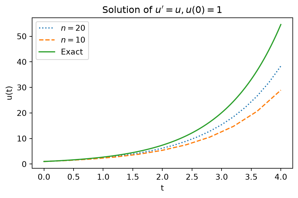
If t is created with np.zeros, t[0] = 0 need not be set explicitly. Setting u[0], however, is essential: forgetting the line u[0] = u0 is a very common error when programming ODE solvers. Figure 4.1 shows the solution for two time steps \(\Delta t\). A smaller \(\Delta t\) improves the approximation, although both solutions are quite inaccurate. With an even smaller time step, the approximation becomes indistinguishable from the exact solution.
4.3 Extending the Solver to General ODEs
As mentioned in Section 4.1, we want to create general solvers that solve any ODE of the form \(u'=f(t,u)\). This requires only a small change to the algorithm above:
- Create arrays
tanduof length \(n+1\) - Set the initial condition:
u[0]\(= u_0\),t[0]\(= 0\) - For \(k=0,1,2,\ldots,n-1\):
t[n+1] = t[n] + dtu[n+1] = u[n] + dt*f(t[n], u[n])
Only the formula that computes u[n+1] from u[n] has changed. In the previous case we had \(f(t,u) = u\). For a general solver we replace u[n] by the more general f(t[n],u[n]). The following Python function implements this generic version of the forward Euler method:
def forward_euler(f, u0, T, N):
    """Solve u'=f(t,u), u(0)=u0, with n steps until t=T."""
    import numpy as np
    t = np.zeros(N+1)
    u = np.zeros(N+1)  # u[n] is the solution at time t[n]

    u[0] = u0
    dt = T/N

    for n in range(N):
        t[n+1] = t[n] + dt
        u[n+1] = u[n] + dt*f(t[n], u[n])

    return t, u
This simple function solves any ODE of the form Equation 4.1. The right-hand side function \(f(t,u)\) is implemented as a Python function and passed to forward_euler together with the initial condition u0, the final time T, and the number of time steps N. From the last two arguments the function computes the time step dt.
To illustrate this, we solve the same problem as above, \(u'=u\), \(u(0)=1\), for \(t\in [0,3]\). The following code uses the function forward_euler for this purpose:
def f(t, u):
    return u

u0 = 1
T = 3
N = 30
t, u = forward_euler(f, u0, T, N)
The function forward_euler returns the two arrays u and t, which we can then plot or process further.
The definition of the right-hand side function f is important. It is always written with the two arguments t and u, even if, as here, only u is used. The solver is meant to work for all ODEs of the form \(u' = f(t,u)\) and therefore calls the function as f(t[n], u[n]). If the right-hand side function were defined as a function of u only, i.e., with def f(u):, this call would fail with an error message. The remedy is simple: write def f(t,u):, even if t never appears inside the function.
For just 15 lines of Python code, forward_euler is remarkably capable. The function solves any linear or nonlinear ODE, including those that cannot be solved analytically. The procedure is always the same: identify \(f(t,u)\) in the ODE, specify the initial condition \(u_0\), implement \(f(t,u)\) as a Python function f(t, u), choose the number of time steps N, call t, u = forward_euler(f, u0, T, N), and plot the solution.
The forward Euler method is the simplest of all ODE solvers. For challenging ODEs there are more accurate and more stable methods. For most ODEs it is nevertheless well suited: if the accuracy is insufficient, one reduces the time step and thereby usually obtains the required accuracy at a negligible increase in computing time.
4.4 The ODE Solver as a Python Class
Implementing the function forward_euler as a Python class makes the solver more flexible. There are many ways to do this. Its use could look like this:
        method = ForwardEuler_v0(f)
        method.set_initial_condition(u0)
        t, u = method.solve(t_span=(0,10),N=100)
        plot(t, u)
The advantages of a class over a function only become apparent once we introduce different solvers. First, we look at what such a solver class needs for the use case above. A constructor (__init__) takes the right-hand side function f as its only argument and stores it as an attribute. The method set_initial_condition takes the initial condition and stores it. The method solve receives the time interval t_span and the number of time steps N, implements the for loop, and returns the solution, similar to the function forward_euler. The time step \(\Delta t\) and the sequences \(t_k\), \(u_k\) must be initialized in one of the methods and can be stored as attributes. Since the time interval and the number of steps are arguments of solve, this is most naturally done there.
In addition, it is convenient to implement advancing the solution by one step as a separate method advance. A new numerical method then typically requires changing only advance. A first version of the solver class could look like this:
import numpy as np

class ForwardEuler_v0:
    def __init__(self, f):
        self.f = f

    def set_initial_condition(self,u0):
        self.u0 = u0

    def solve(self,t_span,N):
        """Compute solution for
        t_span[0] <= t <= t_span[1],
        using N steps."""
        t0,T = t_span
        self.dt = T/N
        self.t = np.zeros(N+1)
        self.u = np.zeros(N+1)

        self.t[0] = t0
        self.u[0] = self.u0

        for n in range(N):
            self.n = n
            self.t[n+1] = self.t[n] + self.dt
            self.u[n+1] = self.advance()
        return self.t, self.u

    def advance(self):
        """Advance the solution one time step."""
        u, dt, f, n, t = self.u, self.dt, self.f, self.n, self.t

        unew = u[n] + dt*f(t[n],u[n])
        return unew
This class performs essentially the same tasks as the function forward_euler. Its main advantage is the flexibility provided by the method advance: for a different numerical method, a new version of advance typically suffices, and the remaining code stays unchanged.
A class is also suitable for the right-hand side \(f(t,u)\), particularly when it contains parameters. An example is the model for logistic growth
\[
u^{\prime}(t)=\lambda u(t)\left(1-\frac{u(t)}{u_{\max}}\right),\quad u(0)=u_0,\quad t\in [0,40].
\tag{4.5}\] It describes the self-limiting growth of a biological population, i.e., growth under limited resources. Initially the population grows approximately exponentially with the growth rate \(\lambda\). As the population size approaches the carrying capacity \(u_{\max}\), the curve flattens out (Figure 4.2). In the code, \(\lambda\) is called alpha and \(u_{\max}\) is R.
The right-hand side contains the two parameters \(\lambda\) and \(u_{\max}\). For our FE function or class, however, it must be implemented as a function of \(t\) and \(u\) alone. A convenient approach is a class with a call method: the parameters are set as attributes in the constructor and used in the method __call__:
class Logistic:
    def __init__(self, alpha, R, u0):
        self.alpha = alpha
        self.R = R
        self.u0 = u0

    def __call__(self, t, u):   # f(t,u)
        return self.alpha*u*(1 - u/self.R)
The main program for logistic growth could look like this:
problem = Logistic(alpha=0.2, R=1.0, u0=0.1)
solver = ForwardEuler_v0(problem)
solver.set_initial_condition(problem.u0)

T = 40
t, u = solver.solve(t_span=(0,T),N=400)
import matplotlib.pyplot as plt
plt.figure(figsize=(10, 6))
plt.plot(t, u, label='u(t)')
plt.title('Solution of the logistic equation')
plt.xlabel('Time (t)')
plt.ylabel('u(t)')
plt.legend()
plt.grid(True)
plt.show()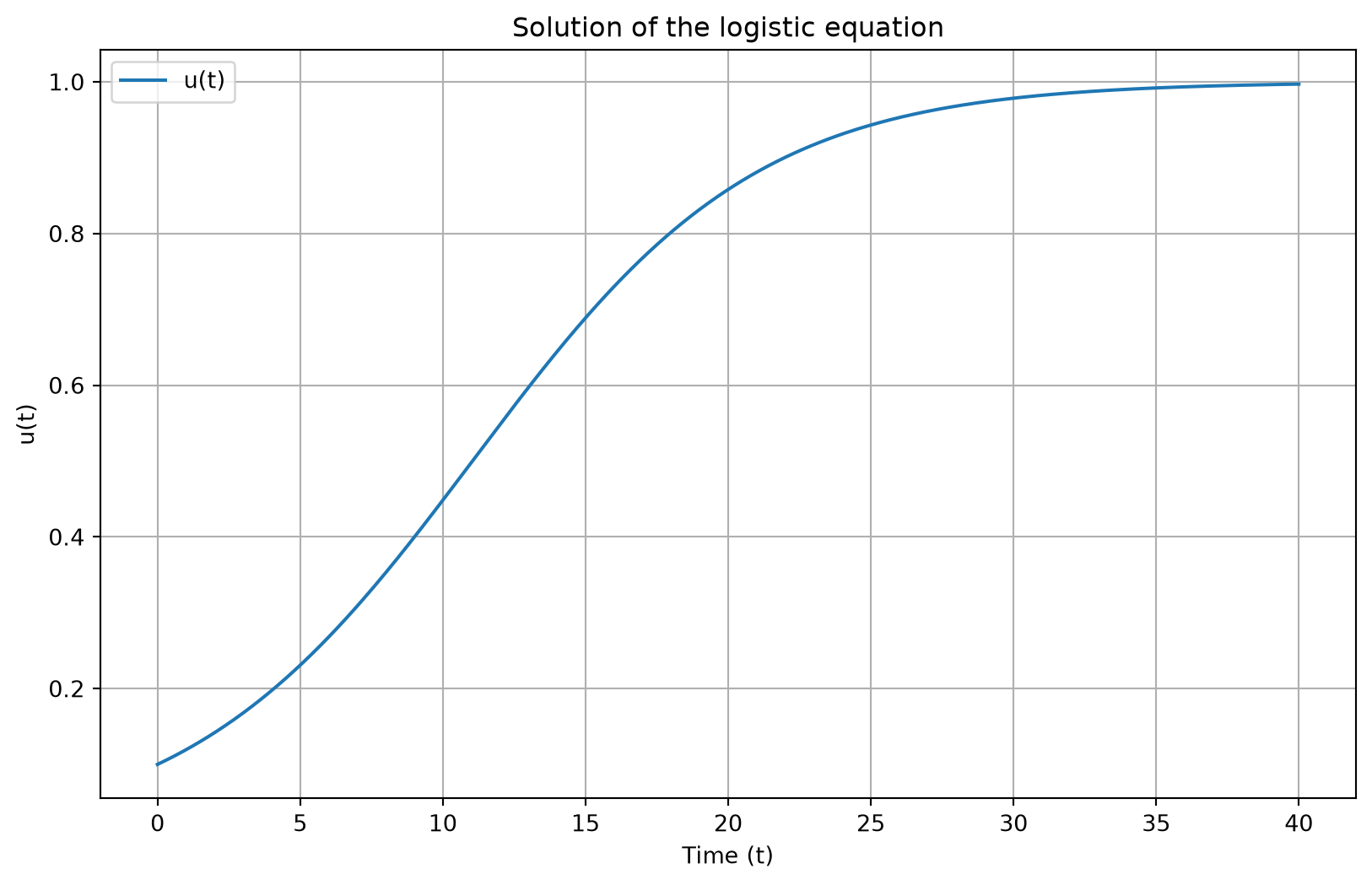
4.5 ODE Systems
So far our ODEs have had a single solution component. They are called scalar ODEs. Many interesting processes are described by systems of ODEs, i.e., by several ODEs in which the right-hand side of one equation depends on the solution of the others. Such systems are also called vector ODEs.
Example 4.2 (System with a Cosine Solution) The system
\[ \begin{alignedat}{2} u' &= v, \quad &&u(0) = 1,\\ v' &= -u, \quad &&v(0) = 0, \end{alignedat} \] has the solution \(u=\cos t\), \(v=-\sin t\). Inserting it into the equations and the initial conditions confirms this.
General ODE systems are usually even harder to solve analytically than scalar ODEs, so numerical methods are needed. In this section we extend the Python programs from Section 4.1 to Section 4.4 to systems of ODEs. Relatively small changes to the code suffice.
The programs should be applicable to any vector ODE and any scalar ODE. To this end, we introduce a general notation.
Definition 4.1 (Vector Form of an ODE System) A system of \(n\) ODEs for the \(n\) unknowns \(u^{(0)}(t), u^{(1)}(t), \ldots, u^{(n-1)}(t)\) has the form
\[ \begin{aligned} \frac{\mathrm{d}}{\mathrm{d}t}u^{(0)} &= f^{(0)}(t, u^{(0)}, u^{(1)}, \ldots, u^{(n-1)}),\\ \frac{\mathrm{d}}{\mathrm{d}t}u^{(1)} &= f^{(1)}(t, u^{(0)}, u^{(1)}, \ldots, u^{(n-1)}),\\ &\;\;\vdots\\ \frac{\mathrm{d}}{\mathrm{d}t}u^{(n-1)} &= f^{(n-1)}(t, u^{(0)}, u^{(1)}, \ldots, u^{(n-1)}). \end{aligned} \] With the solution vector \(u = (u^{(0)}, u^{(1)}, \ldots, u^{(n-1)})\) and the vector-valued right-hand side \(f = (f^{(0)}, f^{(1)}, \ldots, f^{(n-1)})\), the initial value problem in vector form reads
\[ u' = f(t, u),\quad u(t_0) = u_0, \tag{4.6}\] where \(u_0\) is the vector of initial conditions. The superscript \(i = 0, \ldots, n-1\) in \(u^{(i)}\) and \(f^{(i)}\) numbers components, not derivatives.
The function \(f\) has \(n+1\) input arguments (\(t\) and the \(n\) components of \(u\)) and returns a vector of \(n\) values. Equation 4.6 has exactly the same form as Equation 4.3 for scalar ODEs. Whether a scalar ODE or a system is solved is determined solely by \(f\) and the initial condition \(u_0\). This notation is standard in textbooks on ODEs, and the Python implementation can be just as general.
4.6 A ForwardEuler Class for Systems of ODEs
The class ForwardEuler_v0 was written for scalar ODEs. It should now work for a system \(u'=f\), \(u(0)=u_0\), in which \(u\), \(f\), and \(u_0\) are vectors (arrays). To see how the code must be changed, we first consider the numerical method. In the notation of Definition 4.1, the update formula of the forward Euler method looks exactly as in the scalar case, except that all terms are vectors:
\[ \underbrace{u_{k+1}}_{\text{vector}} = \underbrace{u_k}_{\text{vector}} + \Delta t\, \underbrace{f(t_k, u_k)}_{\text{vector}} . \]
Component-wise it reads
\[ u^{(i)}_{k+1} = u^{(i)}_{k} + \Delta t\, f^{(i)}(t_k, u_{k}), \quad i = 0,\ldots , n-1. \]
The compact vector notation, however, is much easier to read. It also corresponds exactly to computing with NumPy arrays. The Python code for the formula can therefore be identical to the version for scalar ODEs,
u[k+1] = u[k] + dt*f(t[k], u[k])with the important difference that u[k] and u[k+1] are now arrays.
The solution u must therefore be a two-dimensional array whose rows are u[k], u[k+1], etc. The function f expects an array as its second argument and returns a one-dimensional array containing all right-hand sides \(f^{(0)},\ldots,f^{(n-1)}\).
What these arrays look like is shown by comparing the solution of a scalar ODE with that of a system of two ODEs.
For a scalar equation, t and u are one-dimensional NumPy arrays. Indexing into u yields numbers, the solution at each time step, for example:
    t = array([0. ,  0.4, 0.8, 1.2, (...) ])
    u = array([1. , 1.4, 1.96, 2.744, (...)])

    u[0] = 1.0
    u[1] = 1.4

    (...)
For a system of two ODEs, t is still one-dimensional. The solution array u, however, is two-dimensional, with one column per solution component. The same indexing now yields a one-dimensional array of length two containing both solution components at one time step:
    u = array([[1.0, 0.8],
               [1.4, 1.1],
               [1.9, 2.7],
                  (...)])

    u[0] = array([1.0, 0.8])
    u[1] = array([1.4, 1.1])

    (...)
The same notation for scalar and vector ODEs and the convenient algebra of NumPy arrays suggest that the solvers for both cases are also very similar. Indeed, after two small changes the class ForwardEuler_v0 from Section 4.4 also works for ODE systems. First, f(t,u) must always return an array. Second, the solver checks whether \(u_0\) is a single number or a list, an array, or a tuple, and creates u as a one- or two-dimensional array accordingly. The second step is not strictly necessary, since a two-dimensional array of size (N+1,1) would also work for scalar ODEs. A one-dimensional array, however, gives simpler and more intuitive indexing. The remaining code from Section 4.4 then works without changes.
The extended class implementation could look as follows:
import numpy as np

class ForwardEuler:
    def __init__(self, f):
        self.f = lambda t,u: np.asarray(f(t,u),float)


    def set_initial_condition(self,u0):
        if isinstance(u0, (float,int)):  #scalar ODE
            self.neq = 1                 #number of eqs.
            u0 = float(u0)
        else:
            u0 = np.asarray(u0)
            self.neq = u0.size
        self.u0 = u0

    def solve(self,t_span,N):
        """Compute solution for
        t_span[0] <= t <= t_span[1],
        using N steps."""
        t0,T = t_span
        self.dt = (T-t0)/N
        self.t = np.zeros(N+1)
        if self.neq == 1:
            self.u = np.zeros(N+1)
        else:
            self.u = np.zeros((N+1,self.neq))

        self.t[0] = t0
        self.u[0] = self.u0

        for n in range(N):
            self.n = n
            self.t[n+1] = self.t[n] + self.dt
            self.u[n+1] = self.advance()
        return self.t, self.u

    def advance(self):
        """Advance the solution one time step."""
        u, dt, f, n, t = self.u, self.dt, self.f, self.n, self.t

        unew = u[n] + dt*f(t[n],u[n])
        return unew
Some parts of this code deserve a comment. The constructor looks almost the same as in the scalar case. However, it uses a lambda function and np.asarray to convert any f that returns a list or a tuple into a function that returns a NumPy array. If f already returns an array, np.asarray passes it through unchanged. This change is not strictly necessary, since one could require the user to return an array. It makes the class more robust and flexible, though. The method set_initial_condition checks whether u0 is a single number (float) or a NumPy array and stores the number of equations in the attribute self.neq. Finally, the method solve checks self.neq and creates u as a one- or two-dimensional array of the appropriate size.
The for loop and the method advance are identical to the previous version of the class.
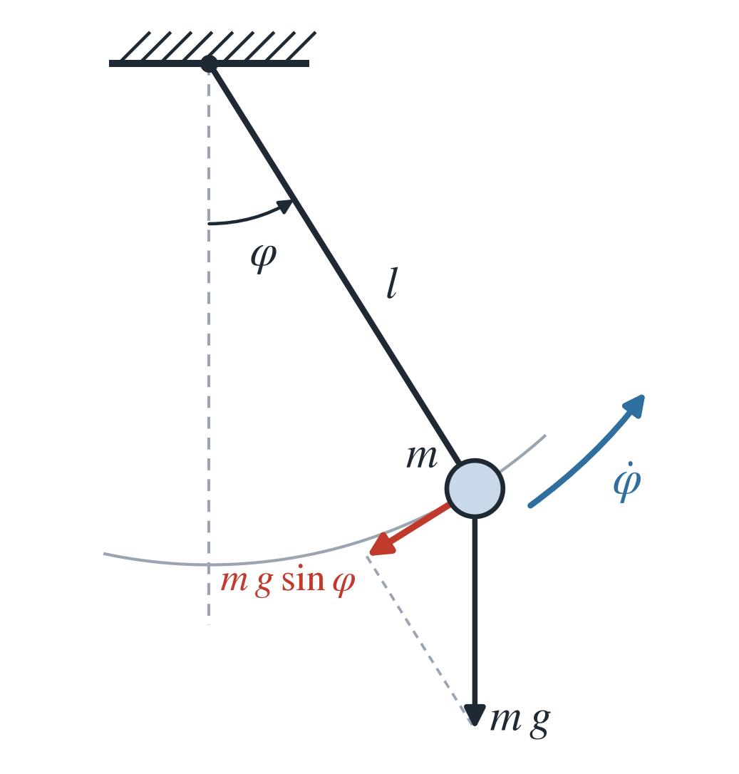
Example 4.3 (ODE Model for a Simple Pendulum) To demonstrate the extended class ForwardEuler, we consider a system of ODEs for the motion of a simple pendulum. This nonlinear system is a classical physical problem and, despite its simplicity, has no exact analytical solution. We formulate it with two variables, the angle of deflection \(\varphi(t)\) and the angular velocity \(\dot{\varphi}(t)\) (Figure 4.3). For a pendulum without friction, we have
\[ \frac{\mathrm{d}}{\mathrm{d}t}\varphi = \dot{\varphi}, \tag{4.7}\]
\[ \frac{\mathrm{d}}{\mathrm{d}t}\dot{\varphi} = -\frac{g}{l}\sin(\varphi) \tag{4.8}\]
with the pendulum length \(l\) and the gravitational acceleration \(g\). Equation 4.7 follows directly from the definition of the angular velocity. Equation 4.8 follows from Newton’s second law: the left-hand side is the angular acceleration \(\ddot{\varphi}\), the right-hand side the tangential component of the weight, divided by the mass and the length of the pendulum. To solve the system, we need initial conditions for both unknowns, i.e., the initial deflection and angular velocity of the pendulum.
The right-hand side of Equation 4.7 and Equation 4.8 contains the parameters \(l\) and \(g\). As for the logistic growth model, we therefore implement it as a class. In the code, \(\varphi\) is called theta, \(\dot{\varphi}\) is omega, and \(l\) is L. A possible implementation:
from math import sin

class Pendulum:
    def __init__(self, L, g = 9.81):
        self.L = L
        self.g = g

    def __call__(self, t, u):
        theta, omega = u
        dtheta = omega
        domega = -self.g/self.L * sin(theta)
        return [dtheta, domega]
The function returns a list. The constructor of the solver class automatically wraps it into a function that returns an array. The main program differs from the previous examples only in the initial condition with two components. The code for the simple pendulum could look like this:
import matplotlib.pyplot as plt

problem = Pendulum(L=1)
solver = ForwardEuler(problem)
theta0, omega0 = np.pi/4, 0
solver.set_initial_condition((theta0,omega0))
T = 10
N = 1000
t, u = solver.solve(t_span=(0,T),N=N)plt.plot(t,u[:,0],label=r'$\varphi$')
plt.plot(t,u[:,1],label=r'$\dot{\varphi}$')
plt.legend()
plt.show()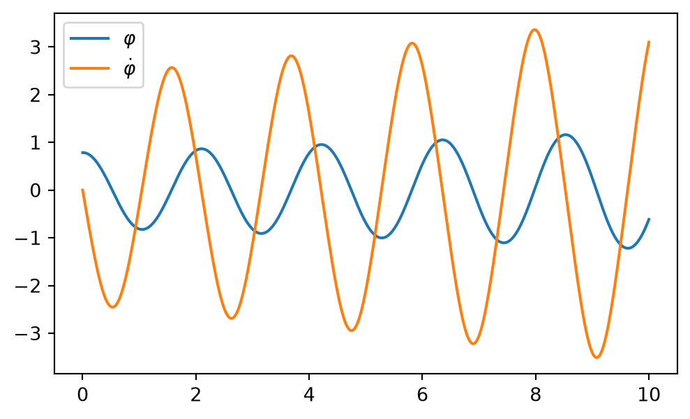
Since u is a two-dimensional array, we extract the individual components by array slicing. In this example, plt.plot(t,u) would also work and plot both solution components. If only selected components are to be plotted, however, slicing is required.
Figure 4.4 shows the result. The labels use Python’s raw string format, indicated by the r in front of the string. Raw strings treat the backslash (\) as a regular character and are therefore convenient for mathematical symbols in LaTeX notation.
The amplitude of the pendulum motion appears to increase with time, which is not physically correct. For the undamped pendulum according to Equation 4.7 and Equation 4.8, energy is conserved, so the amplitude should be constant. The increasing amplitude is a numerical artifact of the forward Euler method. A smaller time step or a different numerical method improves the solution.
4.7 Using ODE Solvers from SciPy
There are numerous ready-made ODE solvers, so implementing our own may seem unnecessary. It is often very useful, however, to know how the solvers we apply work. The best way to learn this is to implement them ourselves.
If, on the other hand, a given ODE model is to be solved as efficiently as possible, several existing solvers are available. For Python programmers, the obvious choice is the solvers from SciPy, which have evolved into a robust and fairly efficient collection. SciPy is an extensive collection of scientific software in Python, with tools for linear algebra, optimization, integration, and other common tasks in scientific computing.
For initial value problems, the function solve_ivp from the module integrate is the tool of choice. The following code uses it to solve the pendulum problem of Equation 4.7 and Equation 4.8 with the class Pendulum, which is stored in the separate file pendulum.py.
from scipy.integrate import solve_ivp
import numpy as np
import matplotlib.pyplot as plt
from pendulum import Pendulum

problem = Pendulum(L=1)
t_span = (0,10.0)
u0 = (np.pi/4, 0)

solution = solve_ivp(problem, t_span, u0)
plt.plot(solution.t, solution.y[0,:])
plt.plot(solution.t, solution.y[1,:])
plt.legend([r'$\varphi$',r'$\dot{\varphi}$'])
plt.show()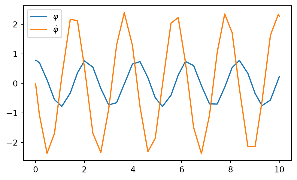
solve_ivp and the default tolerance.
Figure 4.5 shows the result. The solution looks far less smooth than that of the ForwardEuler solver.
The reason for this apparent error is that solve_ivp is an adaptive solver that chooses the time step automatically so that a given error tolerance is met. The default tolerance is relatively large. The solver therefore uses very few time steps, and the curves look jagged.
A comparison with the exact solution shows that the solution at the time points \(t_k\) is quite accurate. Only the linear interpolation between these time points spoils the picture. A smoother plot can be obtained in several ways.
For example, we pass the additional argument t_eval, a NumPy array containing the time points at which the solution is to be evaluated:
t_eval = np.linspace(0,10.0,1001)
solution = solve_ivp(problem, t_span, u0,t_eval=t_eval)
Alternatively, we reduce the error tolerance of the solver, for example as follows:
rtol = 1e-6
solution = solve_ivp(problem, t_span, u0,rtol=rtol)
This call reduces the relative tolerance rtol from its default value 1e-3 (0.001). The absolute tolerance can be adjusted with the parameter atol.
Of the many arguments and options of solve_ivp, we mention only the parameter method, which selects the numerical method. A call like
rtol = 1e-6
solution = solve_ivp(problem, t_span, u0,method='Radau')
replaces the default solver, the explicit embedded Runge-Kutta method of order 5(4) by Dormand and Prince (RK45, in SciPy method='RK45'), with an implicit Radau solver.
A complete description of all parameters of solve_ivp is given in the online documentation of SciPy. Here we present only the most important ones, which suffice for most applications.
Note 4.1: Using
solve_ivp
The solver is called as
solve_ivp(fun, t_span, s0, method = 'RK45', t_eval=None)
with the arguments
fun: right-hand side function of the system,t_span: integration interval \((t_0, t_f)\) with the initial time \(t_0\) and the final time \(t_f\),s0: initial state,method: numerical method, RK45 by default,t_eval: sorted time points int_spanat which the computed solution is stored.
Example 4.4 (Using solve_ivp for \(S' = \cos(t)\)) Consider the ODE \[
\frac{\mathrm{d}S(t)}{\mathrm{d}t}=\cos(t)
\] with the initial value \(S_0 = 0\). The exact solution is \(S(t) = \sin(t)\). We approximate the solution of this initial value problem on the interval \([0, \pi]\) with solve_ivp and plot the approximation and the error (the difference to the exact solution) over time.
import matplotlib.pyplot as plt
import numpy as np
from scipy.integrate import solve_ivp

%matplotlib inline

F = lambda t, s: np.cos(t)

t_eval = np.arange(0, np.pi, 0.1)
sol = solve_ivp(F, [0, np.pi], [0], t_eval=t_eval)

plt.figure(figsize = (12, 4))
plt.subplot(121)
plt.plot(sol.t, sol.y[0])
plt.xlabel('t')
plt.ylabel('S(t)')
plt.subplot(122)
plt.plot(sol.t, sol.y[0] - np.sin(sol.t))
plt.xlabel('t')
plt.ylabel('S(t) - sin(t)')
plt.tight_layout()
plt.show()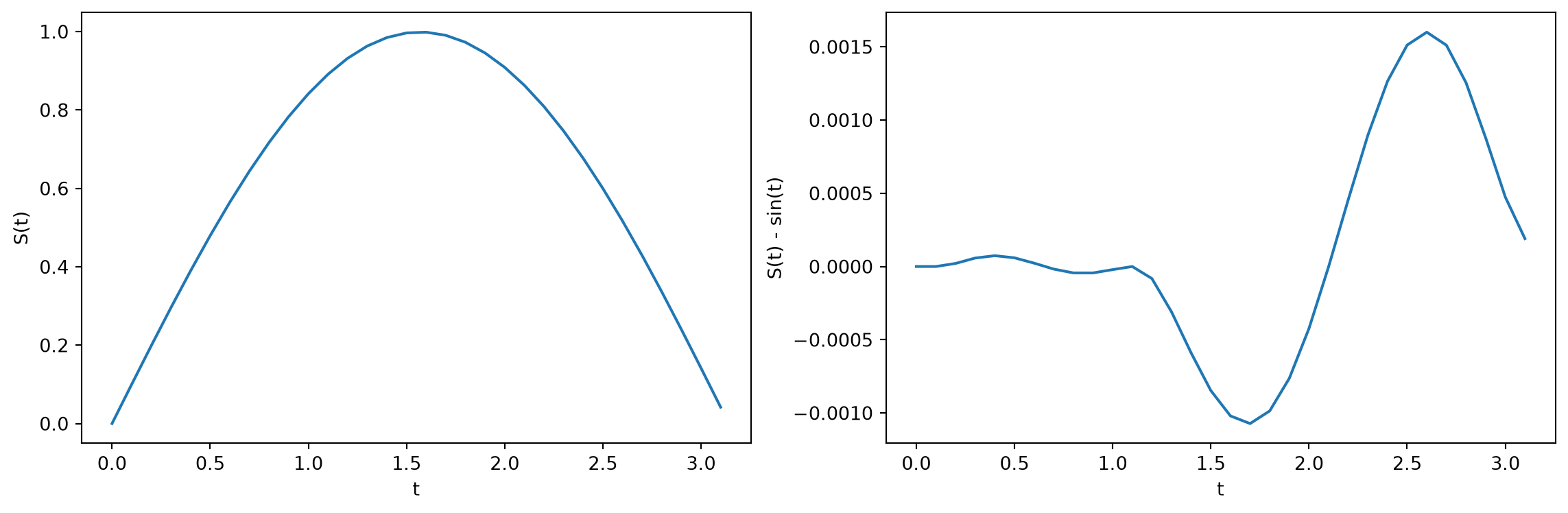
The left figure shows the solution of \(\mathrm{d}S(t)/\mathrm{d}t=\cos(t)\) computed with solve_ivp, the right figure its difference to the analytical solution. The difference is small. The relative and absolute tolerances can be controlled with the arguments rtol and atol. The solver keeps the local error estimates smaller than atol + rtol * abs(S). The default values are 1e-3 for rtol and 1e-6 for atol.
4.8 Exercises
Exercise 4.1 (Using solve_ivp) Use rtol and atol to make the difference between the approximate and the exact solution in Example 4.4 smaller than \(10^{-7}\).
Exercise 4.2 (Exponential Decay with solve_ivp) Consider the ODE
\[ \frac{\mathrm{d}S(t)}{\mathrm{d}t} = -S(t) \]
with the initial value \(S_0 = 1\). The exact solution of this problem is \(S(t) = \mathrm{e}^{-t}\). Use solve_ivp to approximate the solution of this initial value problem on the interval \([0, 1]\). Plot the approximate solution against the exact solution and the error (the difference to the exact solution) over time.
Exercise 4.3 (Using solve_ivp for Coupled Systems) Let the state of a system be defined by
\[ S(t) = \begin{pmatrix} x(t) \\ y(t) \end{pmatrix}, \] and let the behavior of the system be defined by the ODE \[ \frac{\mathrm{d}S(t)}{\mathrm{d}t} = \begin{pmatrix} 0 & t^2 \\ -t & 0 \end{pmatrix} S(t). \]
Use solve_ivp to solve this ODE for the time interval \([0, 10]\) with the initial value \(S_0 = \left[\begin{array}{c} 1 \\1 \end{array}\right]\). Plot the solution in \((x(t), y(t))\).
Exercise 4.4 (Free Undamped Oscillation of a Spring Pendulum) Use solve_ivp to model a spring pendulum that follows the equation of simple harmonic motion
\[ \frac{\mathrm{d}^2x}{\mathrm{d}t^2} = -\frac{c}{m}x \]
Here \(x\) is the displacement of the spring from the equilibrium position (in meters), \(m\) the mass at the end of the spring (in kilograms), and \(c\) the spring constant (in newtons per meter).
Exercise 4.5 (Damped Spring-Mass System) Consider the model of a mass-spring-damper system in one dimension shown in Figure 4.6.
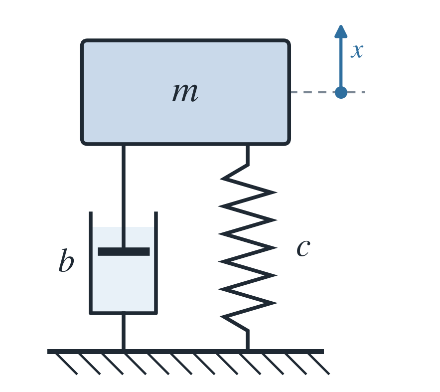
In Figure 4.6, \(m\) denotes the mass of the block, \(b\) the damping constant, and \(c\) the spring constant. A damper dissipates energy by opposing the velocity with a resistance. The damped spring-mass system is a simplified model for engineering applications such as shock absorbers and structural systems.
Acceleration, velocity, and displacement are related by the ODE
\[ m\ddot{x} + b\dot{x} + cx = 0 \] rewritten as \[ \ddot{x}= - \frac{b}{m} \dot{x} - \frac{c}{m} x. \]
The state of the system is described by the vector \(S = [x,\, v]\), where \(x\) is the displacement of the mass from its rest position and \(v\) is its velocity. As a first-order ODE for the state \(S\), the equation reads \[ \frac{\mathrm{d}S}{\mathrm{d}t} = f(t, S). \]
Solve the system with solve_ivp. To this end, define a function my_msd(t, S, m, c, k) with the damping constant \(b\) (c) and the spring constant \(c\) (k). Here \(t\) is a scalar denoting time and \(S\) is a \((2,)\) vector denoting the state of the system. The parameters \(m\), \(b\), and \(c\) are the mass, the damping constant, and the spring constant of the oscillation equation.
Exercise 4.6 (Simple Pendulum: Runge-Kutta Method of Order 4) The (nonlinear) ODE for the motion of a simple pendulum reads \[
\frac{\mathrm{d}^2\varphi}{\mathrm{d}t^2} + \frac{g}{l}\sin(\varphi) = 0,
\] see Figure 2.21 and Equation 2.29. Here \(\varphi = \varphi(t)\) is the angle of deflection of the pendulum from the vertical at time \(t\), \(g\) the gravitational acceleration, and \(l\) the length of the pendulum string. The pendulum is to be deflected from its rest position (\(\varphi(0) = 0\)) and set in motion with an initial angular velocity \(\dot{\varphi}(0) = 1\). For the special case \(g=l\), compute the angle of deflection \(\varphi(t)\) of the pendulum as well as the angular velocity \(\dot{\varphi}\) at time \(t=0.1\) by using a Runge-Kutta method of order 4 from the Python library scipy (function solve_ivp).
4.9 Solutions
Solution 4.1.
sol = solve_ivp(F, [0, np.pi], [0], t_eval=t_eval, \
                rtol = 1e-8, atol = 1e-8)

plt.figure(figsize = (12, 4))
plt.subplot(121)
plt.plot(sol.t, sol.y[0])
plt.xlabel('t')
plt.ylabel('S(t)')
plt.subplot(122)
plt.plot(sol.t, sol.y[0] - np.sin(sol.t))
plt.xlabel('t')
plt.ylabel('S(t) - sin(t)')
plt.tight_layout()
plt.show()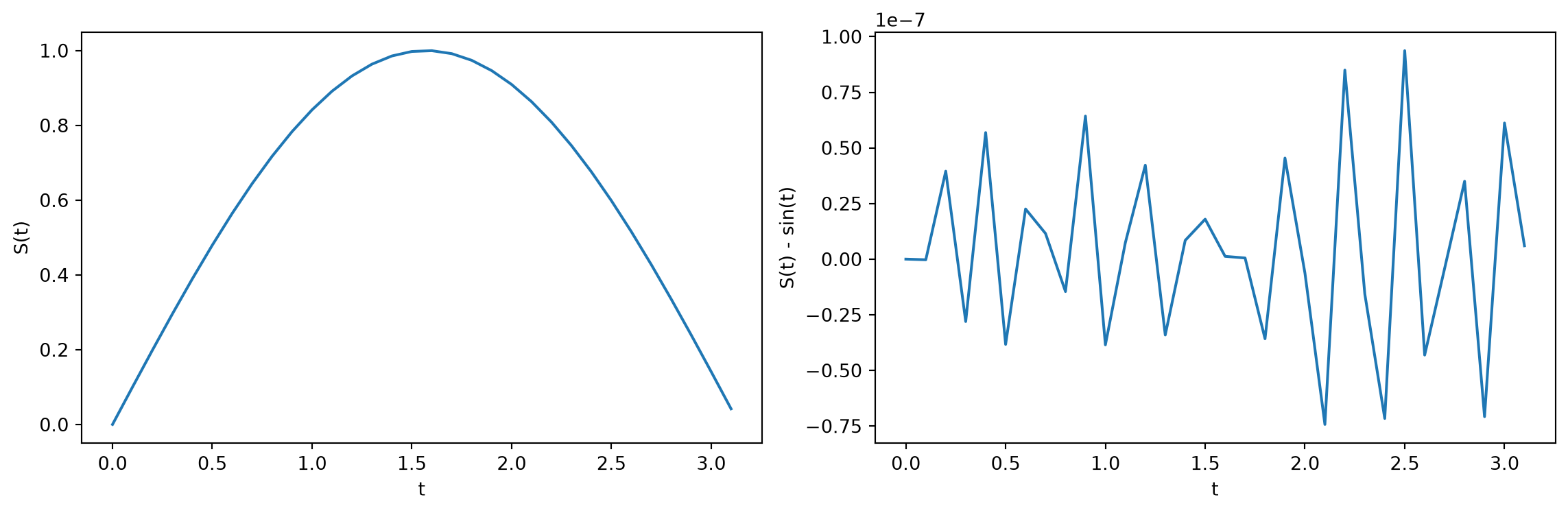
Solution 4.2.
F = lambda t, s: -s

t_eval = np.arange(0, 1.01, 0.01)
sol = solve_ivp(F, [0, 1], [1], t_eval=t_eval)
plt.figure(figsize = (12, 4))
plt.subplot(121)
plt.plot(sol.t, sol.y[0])
plt.xlabel('t')
plt.ylabel('S(t)')
plt.subplot(122)
plt.plot(sol.t, sol.y[0] - np.exp(-sol.t))
plt.xlabel('t')
plt.ylabel('S(t) - exp(-t)')
plt.tight_layout()
plt.show()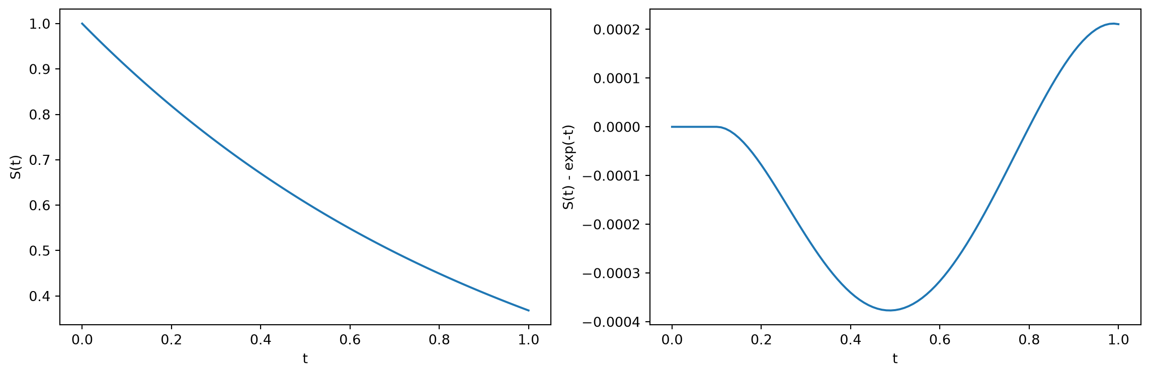
solve_ivp.
Figure 4.7 shows the corresponding numerical results.
Solution 4.3.
F = lambda t, s: np.dot(np.array([[0, t**2], [-t, 0]]), s)

t_eval = np.arange(0, 10.01, 0.01)
sol = solve_ivp(F, [0, 10], [1, 1], t_eval=t_eval)

plt.figure(figsize = (9, 4))
plt.plot(sol.y.T[:, 0], sol.y.T[:, 1])
plt.xlabel('x')
plt.ylabel('y')
plt.show()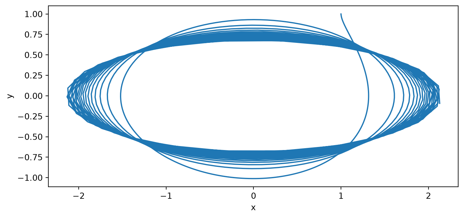
Solution 4.4. Since solve_ivp solves only first-order systems, we transform the second-order equation into a first-order system according to Theorem 2.14. With \(y_1 = x\) and \(y_2 = \mathrm{d}x/\mathrm{d}t\) (y[0] and y[1] in the code), we have
\[ \begin{aligned} \frac{\mathrm{d}y_1}{\mathrm{d}t} & = y_2, \\ \frac{\mathrm{d}y_2}{\mathrm{d}t} & = -\frac{c}{m}y_1. \end{aligned} \]
We solve this system with solve_ivp. For comparison, we plot the exact (analytical) solution of the harmonic oscillation, \[
x(t) = x_0 \cos\left(\omega_0 t + \varphi\right), \quad \omega_0 = \sqrt{\frac{c}{m}},
\] with the amplitude \(x_0\), the spring constant \(c\) (k in the code), the mass \(m\), the time \(t\), and the phase angle \(\varphi\) (cf. Equation 2.9). For the initial velocity \(0\), \(\varphi = 0\), and \(x_0\) equals the initial displacement. The following code implements and visualizes this solution (Figure 4.8).
# Parameters of the spring and the mass
k = 2.0  # spring constant in N/m
m = 0.5  # mass in kg

# The system of first-order differential equations
def federpendel(t, y):
    return [y[1], -k / m * y[0]]

# Initial conditions: initial displacement 1 m, initial velocity 0 m/s
y0 = [1.0, 0.0]

# Time span for the simulation
t_span = (0, 10)

# Solution of the system of differential equations
sol = solve_ivp(federpendel, t_span, y0, t_eval=np.linspace(t_span[0], t_span[1], 1000))

# Computation of the true solution
t_true = np.linspace(t_span[0], t_span[1], 1000)
x_true = y0[0] * np.cos(np.sqrt(k / m) * t_true)plt.figure(figsize=(9, 6))
plt.plot(sol.t, sol.y[0], label='Numerical displacement (m)')
plt.plot(t_true, x_true, 'k--', label='True displacement (m)')
plt.plot(sol.t, sol.y[1], label='Numerical velocity (m/s)')
plt.title('Numerical vs. true solution of the spring pendulum')
plt.xlabel('Time (s)')
plt.ylabel('Displacement / velocity')
plt.legend()
plt.grid(True)
plt.show()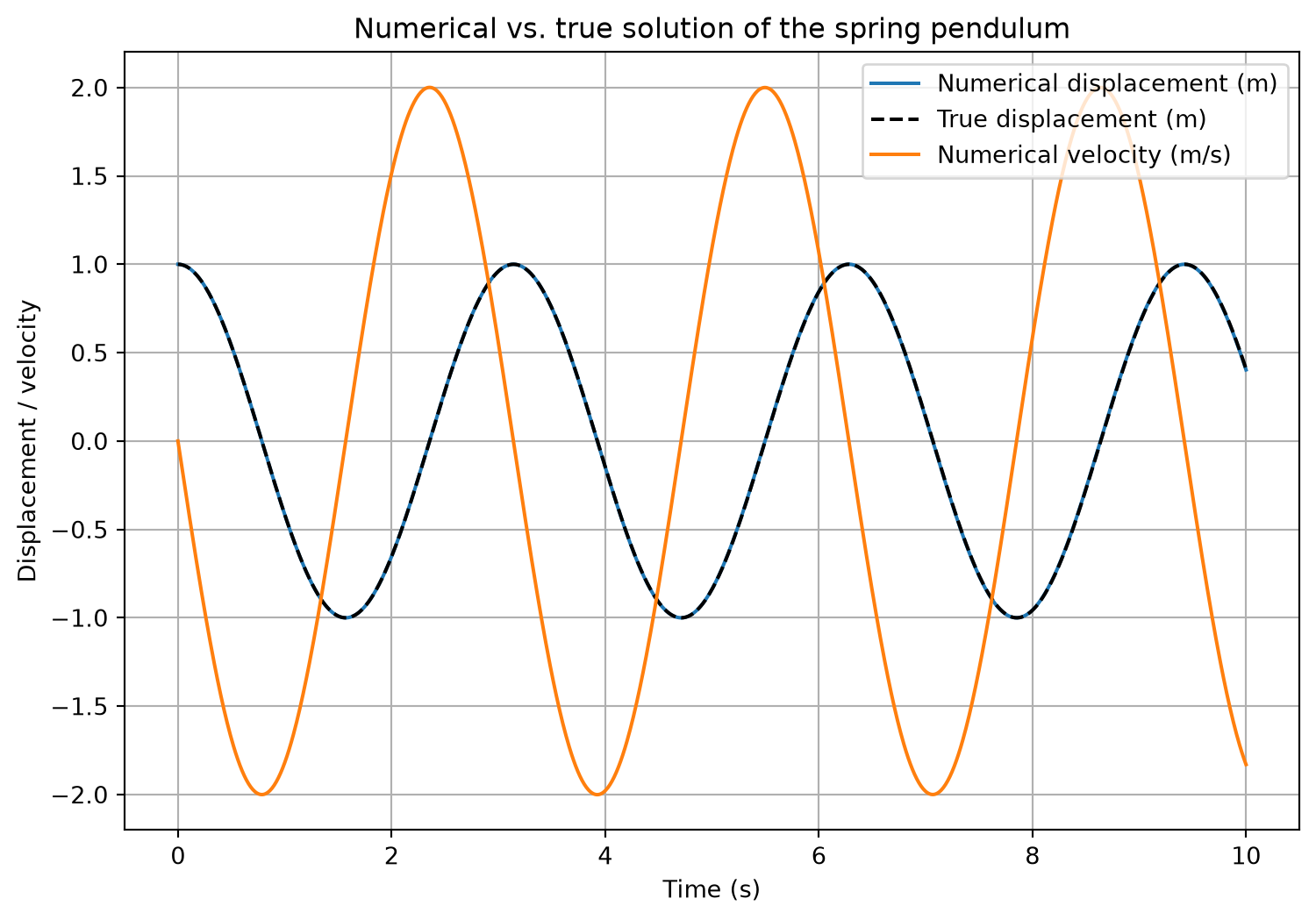
Solution 4.5.
def my_msd(t, S, m, c, k):
    x, v = S # Decompose the state vector S into displacement x and velocity v
    dxdt = v # The derivative of x with respect to time t is v
    dvdt = -(c*v + k*x) / m # The derivative of v with respect to time t
    return [dxdt, dvdt] # Return the derivatives as a list
Here the argument c stands for the damping constant \(b\) and k for the spring constant \(c\). We test the function with \(t=0\), \(S=[1,\, -1]\), \(m=10\), \(b=1\), and \(c=100\):
my_msd(0, [1, -1], 10, 1, 100)[-1, -9.9]Figure 4.9 shows the numerical solution of the spring-mass system for the damping constants \(b = 0\), \(1\), and \(10\) with \(m = 1\) and \(c = 10\).
import numpy as np
from scipy.integrate import solve_ivp
import matplotlib.pyplot as plt
from functools import partial

m = 1
k = 10

# Case 1: no damping
f = partial(my_msd, m=m, c=0, k=k)
t_e = np.arange(0, 20, 0.1)
sol_1=solve_ivp(f,[0,20],[1,0],t_eval=t_e)

# Case 2: weakly damped
f = partial(my_msd, m=m, c=1, k=k)
sol_2=solve_ivp(f,[0,20],[1,0],t_eval=t_e)

# Case 3: strongly damped
f = partial(my_msd, m=m, c=10, k=k)
sol_3=solve_ivp(f,[0,20],[1,0],t_eval=t_e)
plt.figure(figsize = (10, 8))
plt.plot(sol_1.t, sol_1.y[0])
plt.plot(sol_2.t, sol_2.y[0])
plt.plot(sol_3.t, sol_3.y[0])
plt.xlabel('time')
plt.ylabel('displacement')
plt.legend(['No damping', 'Weak damping: $b=1$', \
'Strong damping: $b=10$'], loc=1)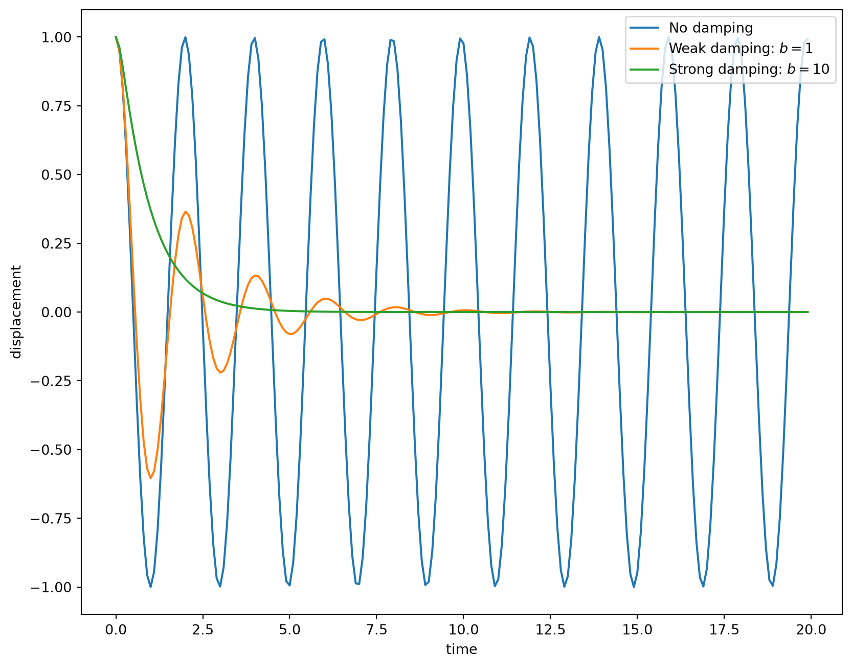
Solution 4.6. With \(g=l\), the ODE for the simple pendulum reads \[ \frac{\mathrm{d}^2\varphi}{\mathrm{d}t^2} + \sin(\varphi) = 0 \] with the initial conditions \(\varphi(0) = 0\) and \(\dot{\varphi}(0) = 1\).
We solve it with solve_ivp from SciPy up to time \(t=0.1\). As its default method, solve_ivp already uses RK45.
First, the second-order ODE is converted into a first-order system. With the angular velocity \(\dot{\varphi}\) as the second unknown (in the code, \(\varphi\) is called phi and \(\dot{\varphi}\) is omega), we have \[
\begin{aligned}
\frac{\mathrm{d}}{\mathrm{d}t}\varphi &= \dot{\varphi}, \\
\frac{\mathrm{d}}{\mathrm{d}t}\dot{\varphi} &= -\sin(\varphi).
\end{aligned}
\]
The following code solves this system, prints \(\varphi(0.1)\) and \(\dot{\varphi}(0.1)\), and plots \(\varphi(t)\) and \(\dot{\varphi}(t)\) for \(0 \le t \le 0.1\) in Figure 4.10.
import numpy as np
from scipy.integrate import solve_ivp
import matplotlib.pyplot as plt

# Define the differential equations
def pendulum_equation(t, y):
    phi, omega = y
    dphi_dt = omega
    domega_dt = -np.sin(phi)
    return [dphi_dt, domega_dt]

# Initial conditions
phi_0 = 0
omega_0 = 1
y0 = [phi_0, omega_0]

# Time interval
t_span = [0, 0.1]
t_eval = np.linspace(t_span[0], t_span[1], 100)  # time points for the output

# Solve the differential equation
solution = solve_ivp(pendulum_equation, t_span, y0, method='RK45', t_eval=t_eval)

# Output the results
phi = solution.y[0]
omega = solution.y[1]

# Print the values for t=0.1
print("phi(t=0.1) =", phi[-1])
print("omega(t=0.1) =", omega[-1])
phi(t=0.1) = 0.09983349976270398
omega(t=0.1) = 0.9950083151697924plt.figure(figsize=[12, 4])
plt.subplot(1, 2, 1)
plt.plot(solution.t, phi, label=r'$\varphi(t)$')
plt.xlabel('t')
plt.ylabel(r'$\varphi(t)$')
plt.legend()
plt.subplot(1, 2, 2)
plt.plot(solution.t, omega, label=r'$\dot{\varphi}(t)$')
plt.xlabel('t')
plt.ylabel(r'$\dot{\varphi}(t)$')
plt.legend()
plt.tight_layout()
plt.show()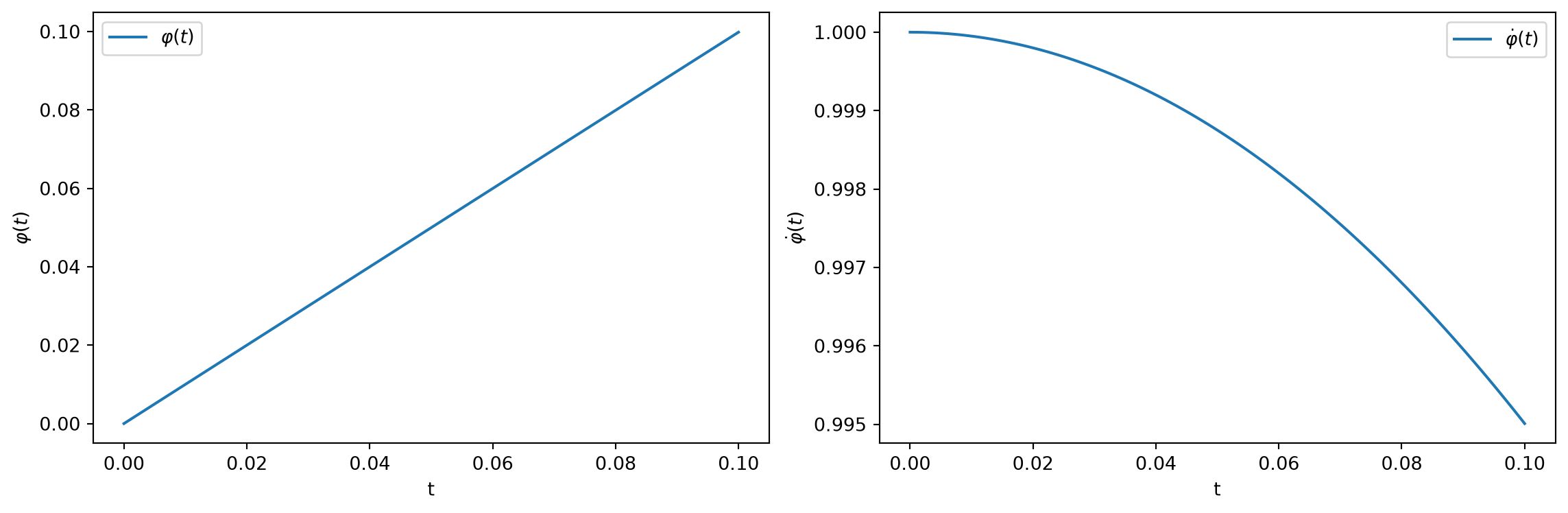
solve_ivp function of SciPy.